A field line's path into the X-line

Advanced level

This page uses Bending flux tubes, The flux function ψ and Reconnection rate and Ohm's law.

Fly a spacecraft across a reconnecting current sheet along \(N\) and you see \(B_L\) fall towards the midplane. Field lines in the inflow region aren't line-tied, so this isn't the stretching from Bending flux tubes. Where does it come from, and what does a single field line do as it comes in?

Why B_L drops towards the midplane

1. \(B_L\) has to pass through zero. The field reverses: \(B_L\approx +B_0\) on one side and \(-B_0\) on the other. Any continuous profile, such as \(B_L = B_0\tanh(N/\delta)\), must cross zero. By Ampère's law that rotation is the current sheet:

\[ \mu_0 J_M = \frac{\partial B_L}{\partial N} - \frac{\partial B_N}{\partial L} \approx \frac{\partial B_L}{\partial N}. \]

The drop in \(|B_L|\) and the current \(J_M\) are the same fact stated two ways.

2. Pressure balance sets the shape. Away from the X-line, field lines are nearly straight along \(L\) (\(\kappa\approx0\)), so the tension term in \(\mathbf{J}\times\mathbf{B}\) is negligible and normal force balance reduces to

\[ \frac{\partial}{\partial N}\left(p + \frac{B^2}{2\mu_0}\right)\approx 0 . \]

Magnetic pressure falls towards the midplane and plasma pressure rises by the same amount. That is why MMS sees enhanced density and temperature at the sheet centre, and why total pressure \(B^2/2\mu_0 + nk_B(T_i+T_e)\) is a standard consistency check on a crossing. (The field lines are not perfectly straight, and their slight bending also makes \(B\) weaker towards the sheet. Section Is the field stronger on the inside of the bend here too? compares the two effects.)

Along vs across field lines

Bending and stretching describe how \(B\) varies along a field line. The \(B_L(N)\) profile describes how \(B\) varies across field lines, from one to the next. Line-tying constrains the first; the current and pressure balance set the second.

3. Flux transport. In steady 2D reconnection, \(E_M\) is uniform and the inflow carries flux at the rate \(E_M = -v_N B_L\). As \(B_L\) weakens towards the midplane, \(|v_N|\) must increase. Flux arrives at the same rate, carried by weaker field moving faster, until frozen-in breaks down in the diffusion region.

How field lines move: the E×B drift

A field line doesn't move along its own length. It moves with the E×B drift. With uniform \(E_M\),

\[ \mathbf{v} = \frac{E_M\hat{\mathbf{M}}\times\mathbf{B}}{B^2}, \qquad v_L = \frac{E_M B_N}{B^2},\quad v_N = -\frac{E_M B_L}{B^2}. \]

• Upstream, \(B_L\) dominates, so the motion is along \(-N\) above the sheet and \(+N\) below: field lines lie along \(L\) but move along \(N\), towards the sheet.
• Downstream, near \(N=0\), \(B_N\) dominates, so the motion turns to \(\pm L\). Only reconnected field lines are carried along \(L\), away from the X-line.
• At the X-line, \(B\to0\) and the drift formally diverges. This is exactly where frozen-in fails.

Flux enters across the top and bottom and leaves across the sides. Nothing enters along \(L\).

The four stages

A simple model is a Harris current sheet of half-thickness \(\delta\) plus a weak, current-free X-point field of strength \(\varepsilon\) (in units where the field far from the sheet is about 1):

\[ \psi = \delta\ln\cosh\!\left(\frac{N}{\delta}\right) + \frac{\varepsilon}{2}\left(N^2 - L^2\right), \qquad B_L = \tanh\!\left(\frac{N}{\delta}\right) + \varepsilon N,\quad B_N = \varepsilon L . \]

Its current is \(\mu_0 J_M = \nabla^2\psi = \mathrm{sech}^2(N/\delta)/\delta\): all of it sits in the sheet, and the field outside is current-free. The figures use \(\delta = 0.3\), \(\varepsilon = 0.1\).

The figure follows field lines in time, from upstream through reconnection. Grey arrows are the E×B drift.

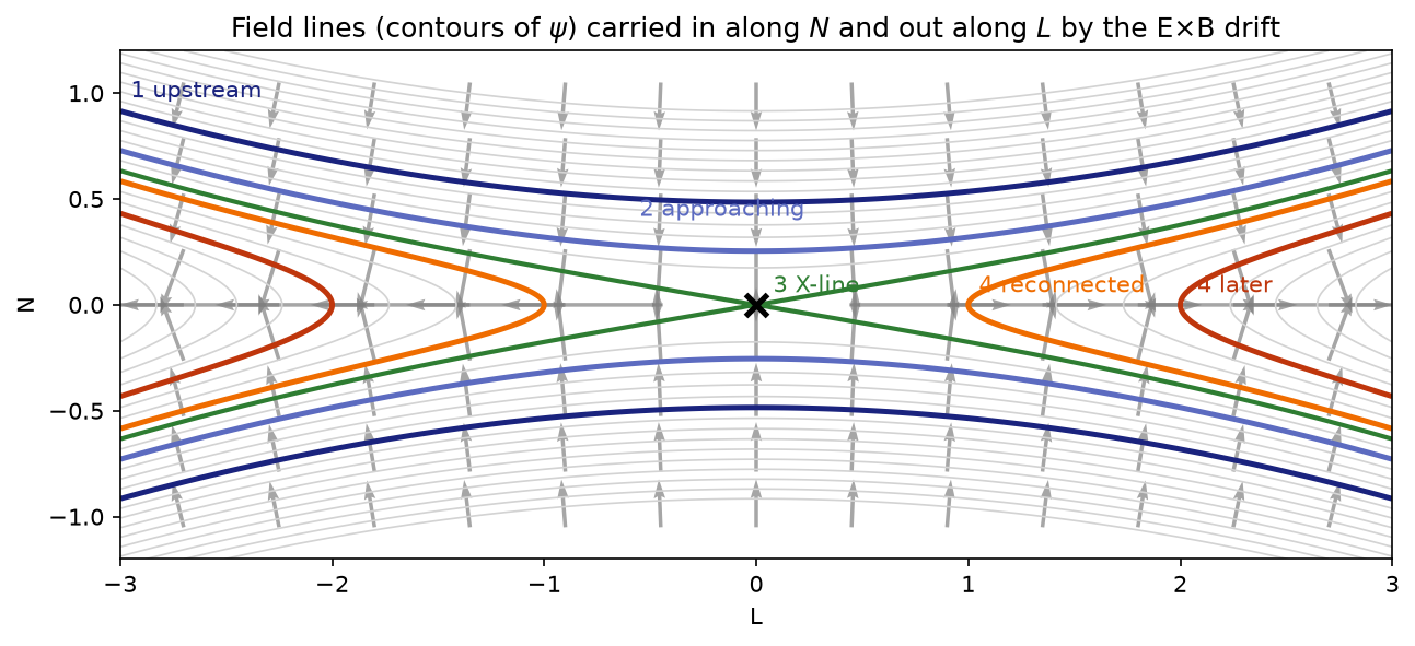
1. Upstream: nearly straight, closely packed. The line runs almost parallel to \(L\) with a slight dip towards the X-line. Contours are close together, so \(B\approx B_0\).

2. Approaching: lines spread apart and dip.

• Spacing. Neighbouring contours are drawn at equal steps \(\Delta\psi\). Since \(\Delta\psi\) is the flux between them, \(B_L\,\Delta n\approx\Delta\psi = \text{const}\), so the gap \(\Delta n\propto 1/B_L\) grows as \(B_L\) drops. The flux tube gets fatter in \(N\): this is the geometric face of the \(B_L\) decrease seen in the data. (In general \(|\mathbf{B}_{\text{in-plane}}|\,\Delta s_\perp\approx\Delta\psi\).)
• Shape. The middle of the line sags towards the X-line while the far parts lag behind, like the bent tube, with the distant parts acting as anchors.
• Forces. The dip is convex towards the sheet, so tension points away from the sheet and resists the inflow. The weaker magnetic pressure at the midplane pushes the line in, and the push wins.

3. At the separatrix: a corner. Curvature at the apex grows without bound. In ideal MHD the line would form a sharp corner at the X-line. In reality frozen-in breaks down at the electron scale \(d_e\), and that is where the line is cut and reconnected.

4. After reconnection: kinked, then straightening. The line now crosses the sheet with \(B_N\ne0\). Its curvature has flipped: tension now points along \(\pm L\), away from the X-line. That is the slingshot. As the kink moves downstream it straightens, and bending energy goes into outflow and heating.

Across the field, spacing grows as \(B\) weakens (pressure balance and flux conservation). Along the field, curvature grows towards the separatrix (bending). The reversal of curvature at reconnection is what turns stored magnetic energy into outflow.

Is the field stronger on the inside of the bend here too?

Question: Bending flux tubes showed that a bent field line has a stronger field on the inside of the bend. Inflowing field lines are bent too. Do they show this, and if so, why does nobody talk about it when describing a current-sheet crossing?

The short answer

Yes, they do. The inside of an inflowing field line's bend is its upstream side, so the rule says \(B\) should be stronger upstream and weaker towards the sheet. That is the same direction as the familiar drop in \(B_L\). The two effects add up; they never contradict each other. But inside the current sheet the field reversal is 10 to 30 times larger, so it hides the bending effect.

Step 1: which side is the inside?

An inflowing field line sags towards the X-line in the middle while its far ends lag behind upstream. Above the sheet it is a shallow ∪. A ∪ curves around a point above it, so:

• the centre of curvature is upstream, far away from the sheet;
• the inside of the bend is the upstream side, and the outside faces the sheet;
• the tension \(B^2\boldsymbol{\kappa}/\mu_0\) points upstream, which is why it resists the inflow.

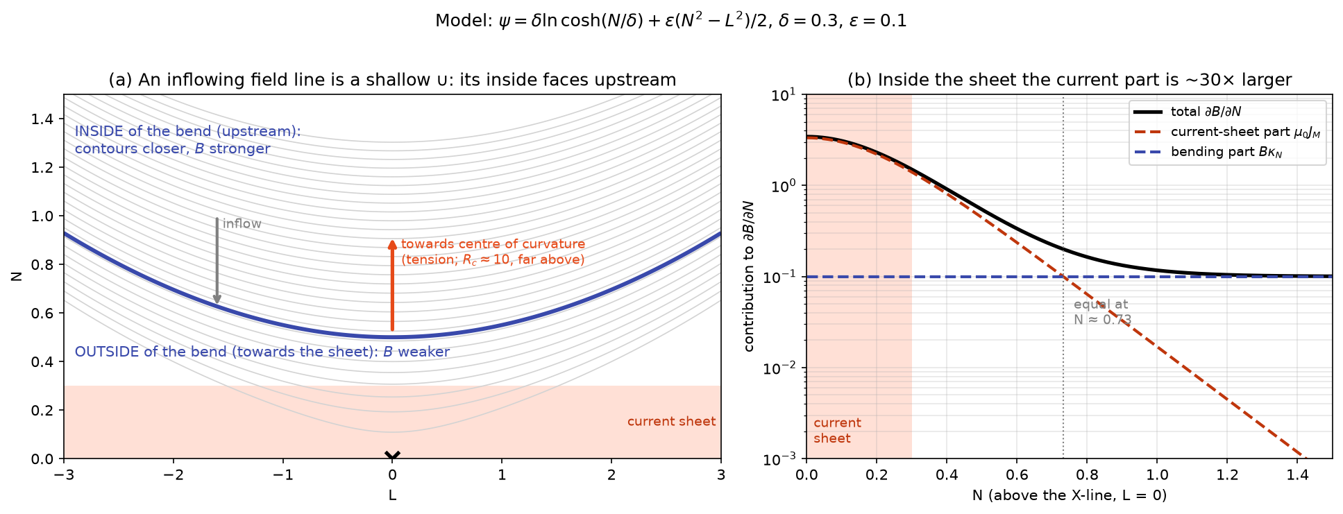
So "stronger on the inside" here means stronger upstream, weaker towards the sheet.

Step 2: split the field gradient into two parts

Look at the field line directly above the X-line (\(L = 0\)). There \(B_N = 0\), so \(B = B_L\) and the line runs along \(L\). Ampère's law gives the current out of the plane:

\[ \mu_0 J_M = \frac{\partial B_L}{\partial N} - \frac{\partial B_N}{\partial L}. \]

The second term is the bending. The field line's slope is \(B_N/B_L\), so its curvature towards \(+N\) is how fast that slope changes along the line: \(\kappa_N = (\partial B_N/\partial L)/B\). Substituting \(\partial B_N/\partial L = B\kappa_N\) and rearranging:

\[ \boxed{\;\frac{\partial B}{\partial N} = \underbrace{B\,\kappa_N}_{\text{bending}} \;+\; \underbrace{\mu_0 J_M}_{\text{current sheet}}\;} \]

The change in field strength across the field line has exactly two sources:

Part	Physical meaning	Size
Bending, \(B\kappa_N = B/R_c\)	The "stronger on the inside" effect. It is the whole gradient when no current flows.	\(\sim B/R_c\)
Current sheet, \(\mu_0 J_M\)	The field reversal. Force balance ties it to plasma pressure: \(p\) rises as \(B\) falls.	\(\sim B/\delta\)

Above the sheet both are positive: each makes \(B\) increase away from the sheet.

Step 3: compare their sizes

For the model above, at \(L = 0\):

\[ \mu_0 J_M = \frac{\mathrm{sech}^2(N/\delta)}{\delta}, \qquad B\kappa_N = \varepsilon . \]

With \(\delta = 0.3\) and \(\varepsilon = 0.1\) (panel b of the figure):

Height above the X-line	Current part	Bending part	Which dominates
\(N = 0\) (midplane)	3.3	0.1	current, ×33
\(N = \delta = 0.3\) (edge of sheet)	1.4	0.1	current, ×14
\(N = 0.6\)	0.24	0.1	current, ×2.4
\(N \approx 0.73\)	0.1	0.1	equal
\(N = 1.0\)	0.017	0.1	bending, ×6

Two regimes appear:

• Inside the current sheet (\(|N|\lesssim 2\delta\)), the current part is much larger. A spacecraft crossing the sheet mostly measures the field reversal. The bending effect is still there, but hidden.
• Far upstream, the current has died away and the field is nearly current-free. The small gradient that remains is almost entirely "stronger on the inside". It is easy to miss because the field changes only slowly there.

The general reason: the bending part scales as \(B/R_c\) and the current part as \(B/\delta\). In the inflow region field lines are only gently curved, so \(R_c\gg\delta\) (here \(R_c\approx10\) versus \(\delta = 0.3\)), and the sheet wins wherever there is a sheet.

Close to the X-line

As a field line approaches the separatrix, its apex sharpens and \(R_c\to 0\). The bending part then grows until it is comparable to the current part, and the clean split above stops being useful. That is also where the fluid picture breaks down and reconnection takes over.

Does plasma pressure change the picture?

No. Force balance across the field line, including the tension term, reads

\[ \frac{\partial}{\partial N}\left(\frac{B^2}{2\mu_0}\right) = \frac{B^2}{\mu_0}\kappa_N - \frac{\partial p}{\partial N}. \]

Above the sheet, \(\kappa_N > 0\) (centre of curvature upstream) and \(\partial p/\partial N < 0\) (pressure peaks at the sheet centre). Both terms are positive, so both make the magnetic field grow upstream.

Check yourself

A field line sits at the edge of a current sheet of half-thickness \(\delta = 500\) km. The field there is \(B = 20\) nT and the field line's radius of curvature is \(R_c = 20\,000\) km. Estimate the ratio of the current part to the bending part of \(\partial B/\partial N\).

Answer

Current part \(\sim B/\delta\), bending part \(\sim B/R_c\), so the ratio is \(R_c/\delta = 20\,000/500 = 40\). The field reversal dominates by a factor of about 40, so the bending effect is invisible in the measured \(B_L\) profile, even though it is there.

Limits of this model

• It is a symmetric Harris sheet plus a uniform X-point field, so the X-line is a simple hyperbolic point. Real fast reconnection has an elongated electron diffusion region and Hall fields (a quadrupolar \(B_M\)); magnetopause reconnection is asymmetric.
• With a guide field, \(|B|\) may barely dip, because \(B_M\) fills in while \(B_L\) reverses. Check \(B_L\), not \(|B|\). And \(\psi\) only describes the in-plane field.
• In slow, collisional (Sweet–Parker-like) regimes, flux can pile up, so \(B_L\) rises in the inflow before dropping. Fast, Hall-mediated reconnection shows little pile-up.

Practice problems

Try each problem before opening its solution. Click an option to check a concept question; type a number and press Check for a numerical one (forms like 6.2e7 or 6.2x10^7 both work).

Concept questions

Problem 1

Upstream of an X-line, in which direction do field lines move?

• Along \(N\), towards the current sheet
• Along \(L\), towards the X-line
• Along \(L\), away from the X-line
• Along \(M\)

Field lines move with the E×B drift. Upstream \(B\approx B_L\hat{\mathbf{L}}\), so \(\mathbf{v}\propto\hat{\mathbf{M}}\times\hat{\mathbf{L}} = -\hat{\mathbf{N}}\): towards the sheet. Nothing comes in along \(L\).

Problem 2

Which side of an inflowing field line's bend is its inside?

• The upstream side, away from the sheet
• The side facing the current sheet
• Neither: the line is straight
• It depends on the guide field

The line sags towards the X-line in the middle, forming a shallow ∪ whose centre of curvature lies upstream.

Problem 3

Inside the current sheet, which part of \(\partial B/\partial N\) dominates?

• The current-sheet part \(\mu_0J_M\)
• The bending part \(B\kappa_N\)
• They are equal
• Neither: \(\partial B/\partial N = 0\) there

The current part scales as \(B/\delta\) and the bending part as \(B/R_c\). In the sheet \(R_c\gg\delta\), so the current part is 10–30 times larger.

Show that…

Problem 4: the drift components

Show that \(\mathbf{v} = E_M\hat{\mathbf{M}}\times\mathbf{B}/B^2\) gives \(v_L = E_MB_N/B^2\) and \(v_N = -E_MB_L/B^2\).

Hint

In a right-handed \((L,M,N)\) system, \(\hat{\mathbf{M}}\times\hat{\mathbf{L}} = -\hat{\mathbf{N}}\) and \(\hat{\mathbf{M}}\times\hat{\mathbf{N}} = \hat{\mathbf{L}}\).

Proof

\(\hat{\mathbf{M}}\times(B_L\hat{\mathbf{L}} + B_N\hat{\mathbf{N}}) = -B_L\hat{\mathbf{N}} + B_N\hat{\mathbf{L}}\). Multiplying by \(E_M/B^2\) gives the two components.

Problem 5: two parts of the gradient

At \(L = 0\), where \(B_N = 0\), show that \(\partial B/\partial N = B\kappa_N + \mu_0J_M\).

Hint

Use Ampère's law for \(J_M\), and \(\kappa_N = (\partial B_N/\partial L)/B\) for the curvature of a line running along \(L\).

Proof

\(\mu_0J_M = \partial_NB_L - \partial_LB_N\). At \(L=0\), \(B = B_L\) and \(\partial_LB_N = B\kappa_N\), so \(\partial_NB = \mu_0J_M + B\kappa_N\).

Numbers

Problem 6

With \(E_M = 1\) mV/m and \(B_L = 20\) nT upstream, how fast do field lines move towards the sheet, in km/s?

Solution

\(|v_N| = E_M/B_L = 10^{-3}/(2\times10^{-8}) = 5\times10^4\) m/s \(= 50\) km/s.

Problem 7

The upstream field is 20 nT and drops to zero at the sheet centre. By how much must the plasma pressure rise from upstream to the centre, in nPa?

Solution

\(\Delta p = B^2/2\mu_0 = (2\times10^{-8})^2/(2\times1.257\times10^{-6}) = 1.59\times10^{-10}\) Pa \(= 0.16\) nPa.

Problem 8

A field line at the sheet edge has \(R_c = 20\,000\) km; the sheet half-thickness is 500 km. Roughly how many times larger is the current part of \(\partial B/\partial N\) than the bending part?

Solution

Current part \(\sim B/\delta\), bending part \(\sim B/R_c\), ratio \(R_c/\delta = 40\).