The Harris current sheet

To study reconnection we need a starting equilibrium with reversing magnetic field. The standard choice is the Harris sheet (Harris, 1962).

The equilibrium

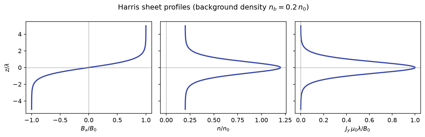
The magnetic field reverses across a layer of half-thickness \(\lambda\):

\[ B_x(z) = B_0 \tanh\!\left(\frac{z}{\lambda}\right), \]

and a dense plasma sits in the middle of the sheet:

\[ n(z) = n_0\,\mathrm{sech}^2\!\left(\frac{z}{\lambda}\right) + n_b, \]

where \(n_b\) is an optional uniform background density.

Pressure balance

In equilibrium, the total pressure (thermal plus magnetic) is constant across the sheet:

\[ n(z)\,k_B (T_i + T_e) + \frac{B_x(z)^2}{2\mu_0} = \text{const}. \]

Using \(\tanh^2 + \mathrm{sech}^2 = 1\), this works out exactly when

\[ n_0 k_B (T_i+T_e) = \frac{B_0^2}{2\mu_0}. \]

The plasma pressure in the middle holds the field apart. The current that supports the field reversal flows out of the page:

\[ J_y(z) = \frac{1}{\mu_0}\frac{dB_x}{dz} = \frac{B_0}{\mu_0\lambda}\,\mathrm{sech}^2\!\left(\frac{z}{\lambda}\right). \]

Coordinate conventions: \((x, y, z)\) vs \((L, M, N)\)

In classic analytic literature (such as Harris 1962), \(x\) is along the reversing field, \(z\) is normal across the sheet (the inflow direction), and \(y\) is the out-of-plane current direction (\(J_y\)).

In the invariant reconnection frame \((L, M, N)\) detailed in the advanced section: - \(L\) is the reconnecting field / outflow axis, - \(N\) is the normal / inflow axis across the sheet, - \(M = N \times L\) is the out-of-plane axis along the sheet current and reconnection electric field.

In the accompanying simulation code splmhd (Cartesian runs), 2D simulations lie in the \((x, y)\) plane: \(x\) corresponds to \(L\) (outflow), \(y\) corresponds to \(N\) (inflow), and \(z\) corresponds to \(M\) (sheet current \(J_z\)). Keep this convention in mind when comparing analytic formulas with simulation arrays!

Triggering reconnection

The Harris sheet is unstable to the tearing mode. In simulations (for example the GEM Reconnection Challenge) we seed it with a small perturbation to the flux function (advanced) \(\psi\), where field lines are contours of \(\psi\):

\[ \psi(x,z) = B_0\lambda \ln\cosh\!\left(\frac{z}{\lambda}\right) + \psi_1 \cos\!\left(\frac{2\pi x}{L_x}\right)\cos\!\left(\frac{\pi z}{L_z}\right). \]

The perturbation creates an X-point at \(x=0\) and magnetic islands (O-points) on either side, just like the island chain on the X-points, O-points and islands page (advanced).

Try it yourself

Run python scripts/make_figures.py and change psi1 in x_point_figure() to see how the size of the island changes.

Practice problems

Try each problem before opening its solution. Click an option to check a concept question; type a number and press Check for a numerical one (forms like 6.2e7 or 6.2x10^7 both work).

Concept questions

Problem 1

Where is the current density of a Harris sheet largest?

• At the centre, \(z = 0\)
• At \(z = \pm\lambda\)
• Far from the sheet
• It is uniform

\(J_y\propto\mathrm{sech}^2(z/\lambda)\), which peaks at \(z=0\), where \(B_x\) changes fastest.

Problem 2

The lobe field \(B_0\) doubles while the temperature stays the same. How must the central density \(n_0\) change to keep pressure balance?

• Double
• Increase four times
• Halve
• Stay the same

\(n_0k_B(T_i+T_e) = B_0^2/2\mu_0\), so \(n_0\propto B_0^2\).

Show that…

Problem 3: pressure balance

Show that \(n(z)k_B(T_i+T_e) + B_x^2/2\mu_0\) is constant across the sheet (with \(n_b = 0\)) if \(n_0k_B(T_i+T_e) = B_0^2/2\mu_0\).

Hint

Use \(\tanh^2u + \mathrm{sech}^2u = 1\).

Proof

\(n_0k_B(T_i+T_e)\,\mathrm{sech}^2 + \dfrac{B_0^2}{2\mu_0}\tanh^2 = \dfrac{B_0^2}{2\mu_0}(\mathrm{sech}^2 + \tanh^2) = \dfrac{B_0^2}{2\mu_0}\), a constant.

Problem 4: the total current

Show that the total current per unit length in \(x\), \(\int_{-\infty}^{\infty}J_y\,dz\), equals \(2B_0/\mu_0\), whatever the thickness \(\lambda\).

Hint

\(J_y = \mu_0^{-1}dB_x/dz\), so the integral is the jump in \(B_x\).

Proof

\(\int J_y\,dz = \mu_0^{-1}[B_x(\infty) - B_x(-\infty)] = \mu_0^{-1}[B_0 - (-B_0)] = 2B_0/\mu_0\). Thinning the sheet raises the peak current but not the total.

Numbers

Problem 5

Magnetotail lobes have \(B_0 = 20\) nT and the sheet plasma has \(k_B(T_i+T_e) = 5\) keV. What central density \(n_0\) gives pressure balance, in cm\(^{-3}\)?

Solution

\(n_0 = B_0^2/(2\mu_0k_B(T_i+T_e)) = 1.59\times10^{-10}/(8.0\times10^{-16})\approx 2\times10^5\) m\(^{-3}\) \(= 0.2\) cm\(^{-3}\).

Problem 6

If the sheet half-thickness is \(\lambda = 1000\) km, what is the peak current density \(J_0 = B_0/(\mu_0\lambda)\), in nA/m²?

Solution

\(J_0 = 2\times10^{-8}/(1.257\times10^{-6}\times10^6) = 1.59\times10^{-8}\) A/m² \(= 15.9\) nA/m².

Problem 7

What is the total current per metre of tail length, \(2B_0/\mu_0\), in A/m?

Solution

\(2\times2\times10^{-8}/1.257\times10^{-6} = 0.032\) A/m, independent of \(\lambda\).