Cartesian runs (2D and 3D)¶

Cartesian geometry is the natural home of the Harris current sheet: a straight sheet of current separating two regions of opposite magnetic field. This page sets up that sheet in the code, shows what a run produces, and gives you a parameter builder to design your own runs. A second setup, a single Alfvén wave, tests that the code solves the equations correctly.

Build your run¶

Choose the setup and the dimensions, change any parameter, and press Download config file. The file goes to your Downloads folder, and the lab finds it there: start the lab and it is listed under Your configs (how to start the lab). The panel on the right updates as you type: it estimates the cost of the run and checks the resolution. Read its warnings before running.

See it before you run it. Above the form is a picture of the chosen setup at \(t = 0\): the magnetic field (in 3D with arrows and field lines), the current, the plasma and the push that starts the run, with what will happen. It is drawn with the example's parameters. Preview script downloads a small Python file that draws the same picture with your parameters: run python3 ~/Downloads/preview_<name>.py (add --html for a 3D page you can rotate). Or type show in the lab before you press Return.

What each parameter means

Parameter	Meaning	Typical range
cells in x, y, z	grid size; doubling every direction costs 8× (2D) or 16× (3D)	64–512
Lx, Ly, Lz	box size in units of \(L_0\) (the sheet half-thickness λ is 0.5)	10–30
resistivity η	\(1/S\): magnetic diffusivity in code units	\(10^{-3}\)–\(10^{-2}\)
viscosity ν	\(1/Re\): kinematic viscosity in code units	about η
extra η at the X-line	a Gaussian bump of resistivity around \(x = y = 0\)	0–0.1
λ	half-thickness of the initial sheet	0.5–1
background density	\(\rho_\infty\), density far from the sheet	0.1–0.3
lobe β	plasma beta far from the sheet	0.1–1
ψ₀	amplitude of the initial X-line perturbation	0.05–0.2
guide field	uniform \(B_z\)	0–1
CFL number	safety factor for the time step	0.3–0.5
filter σ	strength of the grid-noise filter	0.005–0.02

How the code runs¶

The chart follows one run from the config file to the pictures. The boxes in the dashed frames repeat every time step. Click any box to read how that step is done. The live monitor lights up the same stages while your run is going.

2D3D

A 2D run has one cell in z, so every z-derivative is zero. All three components of v, B and A are still evolved (this is often called 2.5D), which is how the out-of-plane current \(J_z\) and a guide field enter.

Coordinate mapping

In splmhd Cartesian runs, \(x\) is along the current sheet (reconnection outflow / \(L\)), \(y\) is normal across the sheet (inflow / \(N\)), and \(z\) is out-of-plane (sheet current \(J_z\) and guide field \(B_z\) / \(M\)). Notice this matches the invariant \((L, M, N)\) frame, with \(y\) taking the role of the normal axis that is often called \(z\) in purely 1D analytical papers (such as the original Harris sheet).

The 3D run has 32 cells in z, periodic in z. Nothing in the code changes: the z-derivatives simply stop being zero. The initial kick is limited to a patch |z| < z_width, so the X-line starts small; whether it spreads is the question.

Setup 1: the Harris sheet¶

Initial state¶

\[ B_x = \tanh\frac{y}{\lambda}, \qquad \rho = \operatorname{sech}^2\frac{y}{\lambda} + \rho_\infty, \qquad p = \tfrac12\operatorname{sech}^2\frac{y}{\lambda} + \tfrac12\beta_\infty . \]

Total pressure \(p + B^2/2 = \tfrac12(1+\beta_\infty)\) is the same everywhere, so this is an exact equilibrium (The Harris current sheet). In the code the field comes from the vector potential \(A_z = \lambda\ln\cosh(y/\lambda)\), so that \(B_x = \partial A_z/\partial y\).

An equilibrium never changes on its own. To start reconnection, the code adds a small perturbation (the same as in the GEM reconnection challenge, Birn et al. 2001):

\[ \delta A_z = \psi_0\cos\frac{2\pi x}{L_x}\cos\frac{\pi y}{L_y}. \]

It pinches the field lines together at \(x = 0\), making an X-line there and O-lines at \(x = \pm L_x/2\). In 3D it can be multiplied by \(e^{-(z/w_z)^2}\), so the X-line starts as a patch of width \(w_z\).

splmhd/setups.py

def harris(grid, prm):
    """Harris current sheet in the x-z plane with a GEM-style perturbation.

    B_x = tanh(y/lam),  rho = sech^2(y/lam) + rho_inf,  p = 0.5 sech^2 + p_inf.
    Total pressure p + B^2/2 is uniform, so the sheet is in equilibrium.
    A_z = lam ln cosh(y/lam) gives B_x = dA_z/dy.
    The perturbation dA_z = psi0 cos(2 pi x/Lx) cos(pi y/Ly) puts an X-line at x = 0.
    """
    if grid.geometry != "cartesian":
        raise ValueError("the Harris setup needs cartesian geometry")
    lam = prm.get("lam", 0.5)
    rho_inf = prm.get("rho_inf", 0.2)
    beta_inf = prm.get("beta_inf", 0.2)  # plasma beta in the lobes, 2 p_inf / B0^2
    psi0 = prm.get("psi0", 0.1)
    z_width = prm.get("z_width", 0.0)   # 3D: localize the perturbation in z (0 = uniform)
    noise = prm.get("noise", 0.0)       # random velocity noise, breaks the symmetry
    x, y, z = grid.X
    Lx, Ly = grid.hi[0] - grid.lo[0], grid.hi[1] - grid.lo[1]

    s = _blank(grid)
    sech2 = 1.0 / np.cosh(y / lam) ** 2
    s["rho"] = sech2 + rho_inf
    s["p"] = 0.5 * sech2 + 0.5 * beta_inf
    shape_z = np.exp(-(z / z_width) ** 2) if (z_width > 0 and grid.active[2]) else 1.0
    A_eq = np.zeros_like(s["A"])
    A_eq[2] = lam * np.log(np.cosh(y / lam))
    s["A"][2] = A_eq[2] + psi0 * np.cos(2 * np.pi * x / Lx) * np.cos(np.pi * y / Ly) * shape_z
    if noise > 0:
        rng = np.random.default_rng(prm.get("seed", 1))
        s["v"] += noise * rng.standard_normal(s["v"].shape) * np.exp(-(y / (2 * lam)) ** 2)
    extra = {"B_bg": np.array([0.0, 0.0, prm.get("b_guide", 0.0)]), "A_eq": A_eq}
    return s, extra

Boundaries. Periodic in \(x\) (and \(z\)); conducting walls at \(y = \pm L_y/2\).

What happens¶

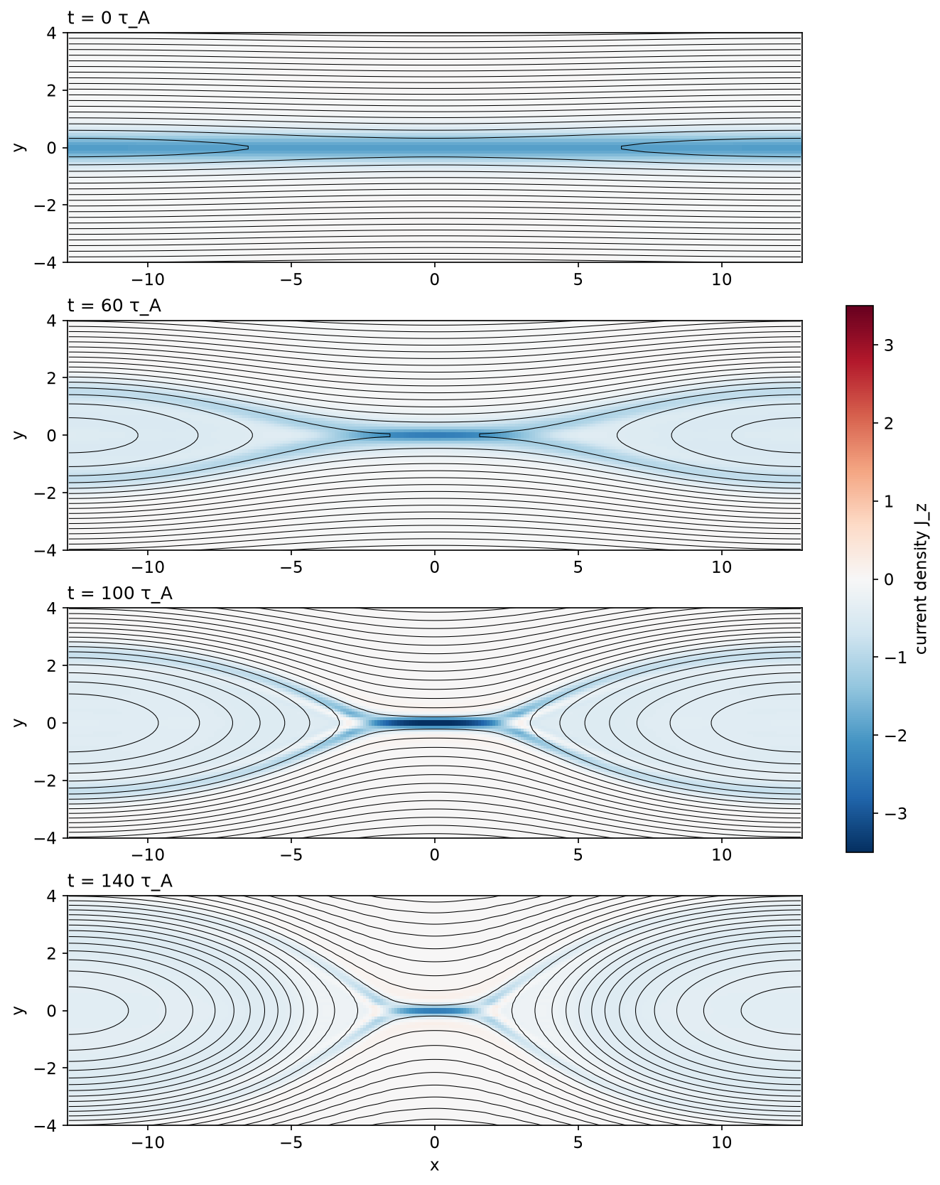
Current density and field lines of the 2D Harris run

The pictures are snapshots of cartesian_2d_harris (\(\eta = \nu = 5\times10^{-3}\), \(256\times128\) cells). Colour is the current density \(J_z\); black lines are contours of \(A_z\), which are field lines because \(A_z\) is the flux function ψ.

\(t = 0\). A straight sheet, slightly pinched at \(x = 0\).
Thinning (\(t\approx 60\)). The inflow presses field lines into the X-line. The current concentrates in a thin sheet that grows longer: a Sweet–Parker sheet.
Fast phase (\(t\approx100\)). Reconnected field lines, sharply bent, shoot out sideways at close to the Alfvén speed. These are the outflow jets, driven by magnetic tension. They feed the growing magnetic islands at \(x = \pm L_x/2\).
Saturation (\(t\approx150\)). Most of the available flux has been reconnected; the island fills the box and the sheet disappears.

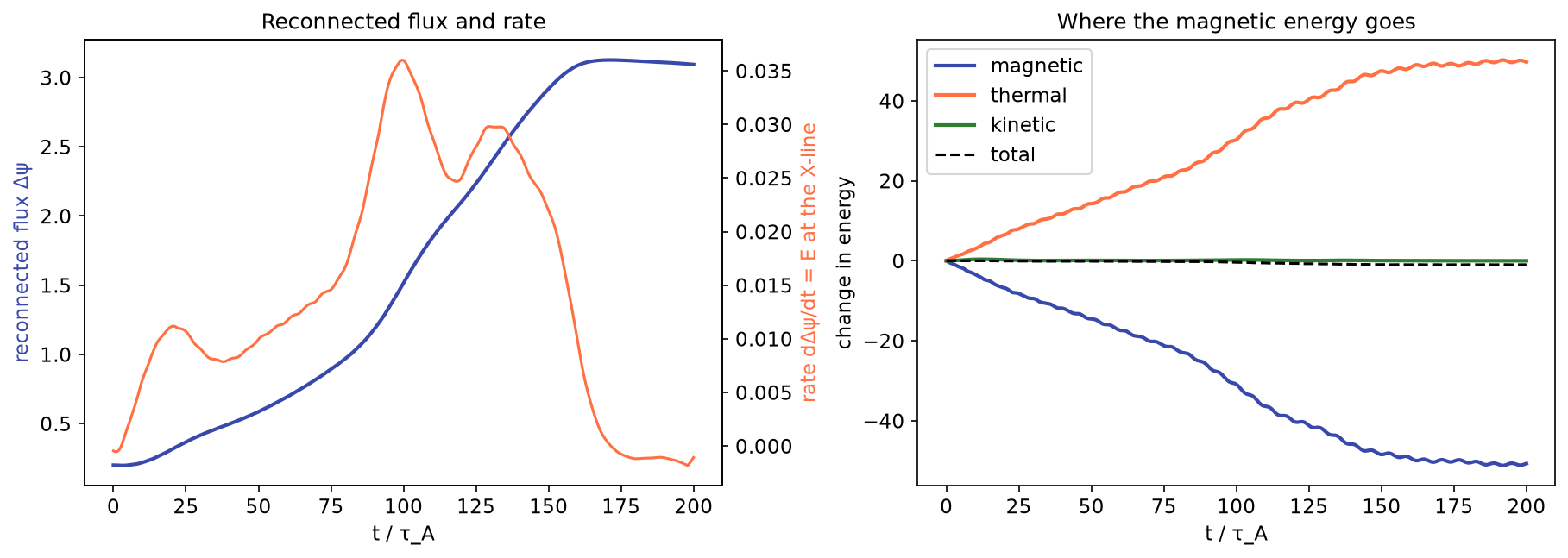
Reconnected flux, rate and energy budget

Reconnection rate. The reconnected flux \(\Delta\psi\) is the difference between \(A_z\) at the X-line and at the O-line: the flux inside the island. Its rate of change is the electric field at the X-line (why). It peaks at about 0.035. The Sweet–Parker estimate with \(L = L_x/2 = 12.8\) is \(S = L/\eta \approx 2600\) and rate \(S^{-1/2}\approx 0.02\), so the simulation and the theory agree to within a factor of 2. That is as close as such an order-of-magnitude model can be expected to get.

Energy. Magnetic energy falls by about 50 units, and almost all of it ends up as heat. Kinetic energy stays small: the jets carry energy to the islands, where viscosity and compression turn it into heat. Total energy changes by less than 0.5%, the size of the numerical error.

Experiments to try¶

1. Is the rate really proportional to η^1/2?

Run with \(\eta = \nu = 0.0025, 0.005, 0.01\) and compare the peak rates in timeseries.png. Sweet–Parker predicts the rate to grow by \(\sqrt2\) each time \(\eta\) doubles. At \(\eta = 0.0025\) the builder warns that the sheet is under-resolved: use \(512\times256\) cells (about 30 minutes).

2. Localized resistivity: Petschek-like fast reconnection

Set extra η at the X-line to 0.02 with width 1. The diffusion region can no longer stretch into a long Sweet–Parker sheet; it stays short, and the outflow opens into a wedge bounded by slow shocks, as in the Petschek model. In our test the reconnected flux reached 2.3 by \(t = 30\), against 0.4 with uniform \(\eta\): about six times faster.

With 0.05 the jets reach the lobe Alfvén speed (\(1/\sqrt{\rho_\infty}\approx 2.2\)) and form shocks, which central differences handle badly: the run crashes after about 20 Alfvén times. Raising ν to 0.02 and the filter to 0.02 keeps it stable (peak rate about 0.13, four times the Sweet–Parker value).

3. A guide field

Set the guide field to 1. Field lines now reconnect at an angle; the out-of-plane field is compressed in the islands and the outflow is slower. Look at B3 and v3 with plot_fields.py --fields B3,v3.

4. High Lundquist number: plasmoids

Theory and research simulations show that above \(S\approx10^4\) a long Sweet–Parker sheet becomes unstable and breaks up into a chain of small islands, plasmoids. Try \(\eta = \nu = 10^{-3}\) (\(S\approx1.3\times10^4\)) with at least \(512\times256\) cells and a small noise (add "noise": 0.01 to setup_params). This takes a few hours on a laptop; whether you see plasmoids depends on the resolution. That is a real lesson about simulations.

3D: a patchy X-line¶

In 3D (cartesian_3d_harris, \(128\times64\times32\) cells, about 15 minutes) the initial perturbation is confined to a patch \(|z|\lesssim 2.5\) of a sheet that is 16 units long in \(z\). Each column below is one time; the top row shows the reconnection electric field \(E_z\) in the middle of the sheet and the bottom row the outflow \(v_x\), both in the \(x\)–\(z\) plane through \(y = 0\):

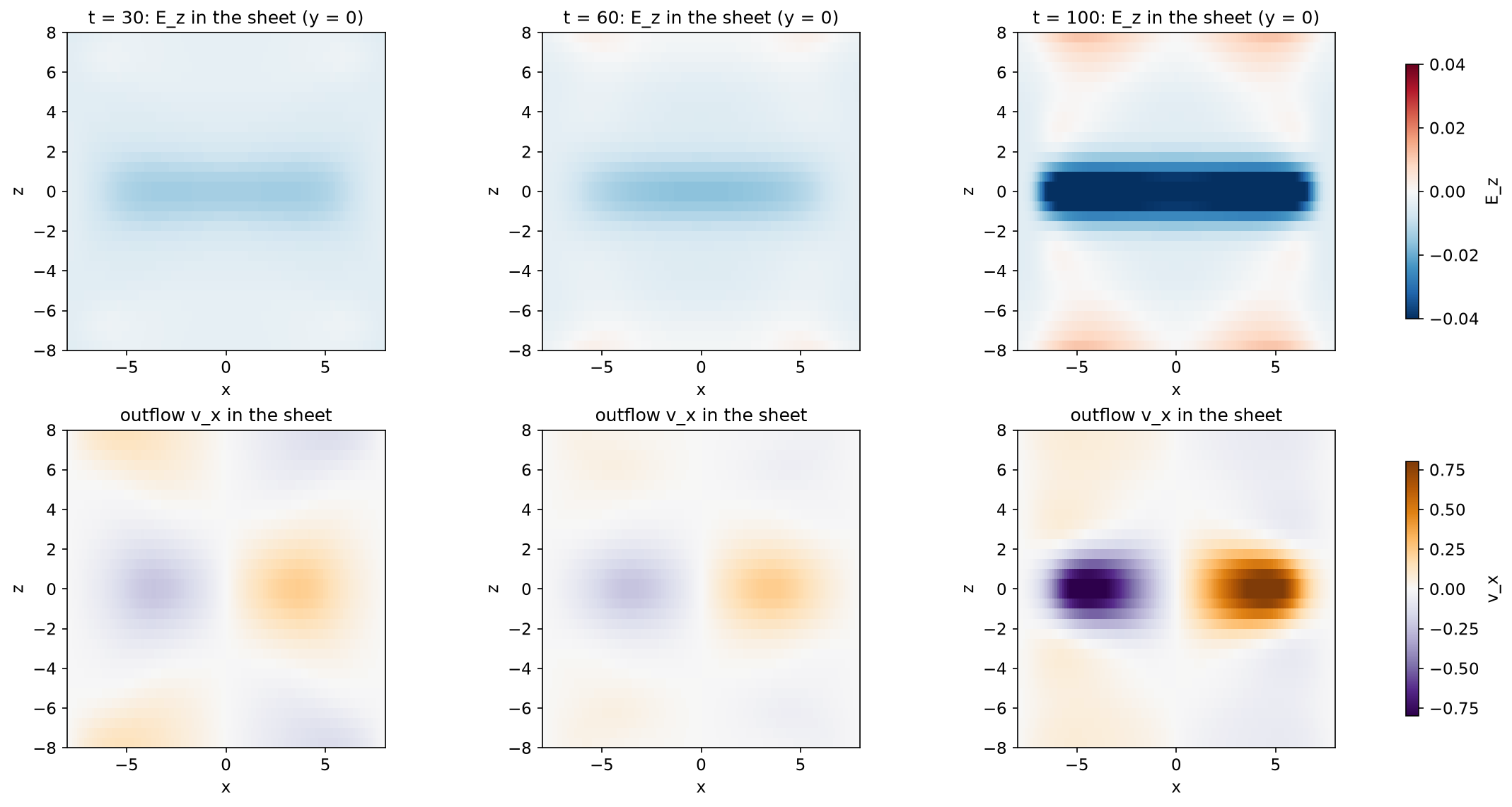
A localized X-line in 3D: reconnection electric field and outflow in the plane of the sheet

What the run shows. Reconnection stays where it started. By \(t = 100\) the electric field at the X-line is about ten times stronger in the patch than at \(|z| = 8\), and the jets are confined to \(|z|\lesssim 2\). The rest of the sheet hardly reconnects at all.

Why this is interesting. Spacecraft observe reconnection X-lines in the magnetotail that start small and then spread along the current direction, by thousands of kilometres. In resistive MHD nothing pushes the X-line sideways: the edges of the patch only grow by slow diffusion. In real plasmas the spreading comes from physics that resistive MHD leaves out. The ions and electrons that carry the current drift along \(z\) and carry the X-line with them, which is the Hall physics of the generalized Ohm's law. Comparing the two is an example of using a simulation to find out what a model is missing.

Try it: make the patch wider (z_width = 6) or remove it (0, a 2D-like X-line) and compare the reconnected flux. Use tools/view3d.py to see the field lines in 3D, and ParaView for isosurfaces.

Setup 2: the Alfvén-wave test¶

A uniform field \(\mathbf{B}_0 = \hat{\mathbf{x}}\) carries a small transverse wave, \(v_z = a\sin kx\), \(B_z = -a\sin kx\). The exact solution travels at \(v_A = 1\) without changing shape, and its energy decays as \(e^{-(\eta+\nu)k^2t}\). The default run (64 cells per wavelength) matches this to 0.3% (figure). Try 16 or 8 cells per wavelength and watch the error grow as \(\Delta x^2\): the second-order accuracy of central differences, measured.

Practice problems¶

Try each problem before opening its solution. Click an option to check a concept question; type a number and press Check for a numerical one (forms like 6.2e7 or 6.2x10^7 both work).

Concept questions¶

Problem 1

Why does the Harris setup need an initial perturbation \(\delta A_z\)?

To make the field divergence-free
An exact equilibrium does not evolve; something must start the X-line
To satisfy the wall boundary conditions
To add the resistivity

The sheet is in force balance, so without a perturbation nothing would happen apart from slow resistive diffusion. The perturbation chooses where the X-line forms.

Problem 2

Where does most of the released magnetic energy end up in the 2D Harris run?

Kinetic energy of the outflow jets
It leaves through the walls
Thermal energy (heat)
Gravitational energy

The jets carry energy only temporarily. Ohmic heating in the sheet, and viscous and compressive heating in the islands, turn almost all of it into heat. Kinetic energy remains small throughout.

Problem 3

How can you read the reconnection rate from the simulation?

As \(d\Delta\psi/dt\), equal to the electric field \(E_z\) at the X-line
As the maximum flow speed
As the maximum current density
As the total magnetic energy divided by time

In 2D, \(\partial_tA_z = -E_z\), so the change of \(A_z\) at the X-line per unit time is the out-of-plane electric field there: the flux reconnected per unit time.

Show that…¶

Problem 4: the Harris sheet is in equilibrium

Show that \(p + B_x^2/2\) is uniform for \(B_x = \tanh(y/\lambda)\) and \(p = \tfrac12\operatorname{sech}^2(y/\lambda) + \tfrac12\beta_\infty\).

Hint

Use \(\tanh^2 + \operatorname{sech}^2 = 1\).

Proof

\(p + B_x^2/2 = \tfrac12\operatorname{sech}^2 + \tfrac12\beta_\infty + \tfrac12\tanh^2 = \tfrac12(1 + \beta_\infty)\), a constant. In 1D the momentum equation is \(\partial_y(p + B^2/2) = 0\) (field lines are straight, so there is no tension), so the sheet is in equilibrium.

Problem 5: where the X-line is

Show that with \(\delta A_z = \psi_0\cos(2\pi x/L_x)\cos(\pi y/L_y)\), \(A_z\) along \(y = 0\) has a maximum at \(x = 0\) and minima at \(x = \pm L_x/2\). Why does this make \(x = 0\) an X-line?

Hint

Across the sheet (in \(y\)), \(A_z = \lambda\ln\cosh(y/\lambda)\) has a minimum at \(y = 0\). A point that is a minimum one way and a maximum the other is a saddle.

Proof

Along \(y = 0\), \(A_z = \psi_0\cos(2\pi x/L_x)\): maximum at \(x = 0\), minimum at \(\pm L_x/2\). Across the sheet \(A_z\) has a minimum at \(y = 0\). So \(x = 0\) is a saddle of \(A_z\) (an X-point), and \(x = \pm L_x/2\) are minima in both directions (O-points), as on the X- and O-points page.

Numbers¶

Problem 6

The default 2D Harris run has \(L_x = 25.6\) and \(\eta = 5\times10^{-3}\). Using \(L = L_x/2\), what Sweet–Parker reconnection rate \(S^{-1/2}\) do you expect?

Solution

\(S = 12.8/0.005 = 2560\), so \(S^{-1/2} = 0.0198\). The simulation's peak rate, about 0.035, is within a factor of 2.

Problem 7

With the same numbers, how thick is the Sweet–Parker sheet, \(\delta = LS^{-1/2}\)? How many cells is that with \(\Delta y = 0.1\)?

Solution

\(\delta = 12.8\times0.0198 = 0.253\), only about 2.5 cells. The sheet is barely resolved, which is why the filter is needed.

Problem 8

In physical units, take \(L_0 = 1000\) km and \(v_A = 1000\) km/s (magnetotail-like). How many seconds is the Harris run's \(t = 200\,\tau_A\)?

Solution

\(\tau_A = L_0/v_A = 1\) s, so \(t = 200\) s, a little over 3 minutes. Because the equations are dimensionless, the same run also describes a solar flare, with \(\tau_A\sim10\) s.