Simulation Lab

The pages so far derive reconnection with pencil and paper. Here you run it. The Simulation Lab is a small resistive-MHD code, splmhd, that solves the equations derived in Resistive MHD: deriving the equations on a grid, in Cartesian or spherical coordinates, in 2D or 3D.

The code is written in plain Python and NumPy so that you can read every line. These pages explain how the equations become code; your laptop does the computing.

How it works

1. Download the code (once): one zip file with the solver, example runs and plotting tools.
2. Double-click Start Lab in the unzipped folder. The first time, it installs numpy and matplotlib for itself.
3. Pick a run from the menu, or a config file you made with the parameter builders on the Cartesian and Spherical pages.
4. Watch it live: one window shows each stage of the algorithm, the energy budget, the reconnection rate and the checks; four more show the magnetic field, the current, the flow and the plasma as the run goes. At the end the plots and a movie are made for you; 3D runs can open ParaView.

⬇ Download splmhd.zip (57 kB)

New to running code? Run it on your computer walks through every step: where the download goes, how to unzip it, where to keep the folder, how to start the lab and what you will see.

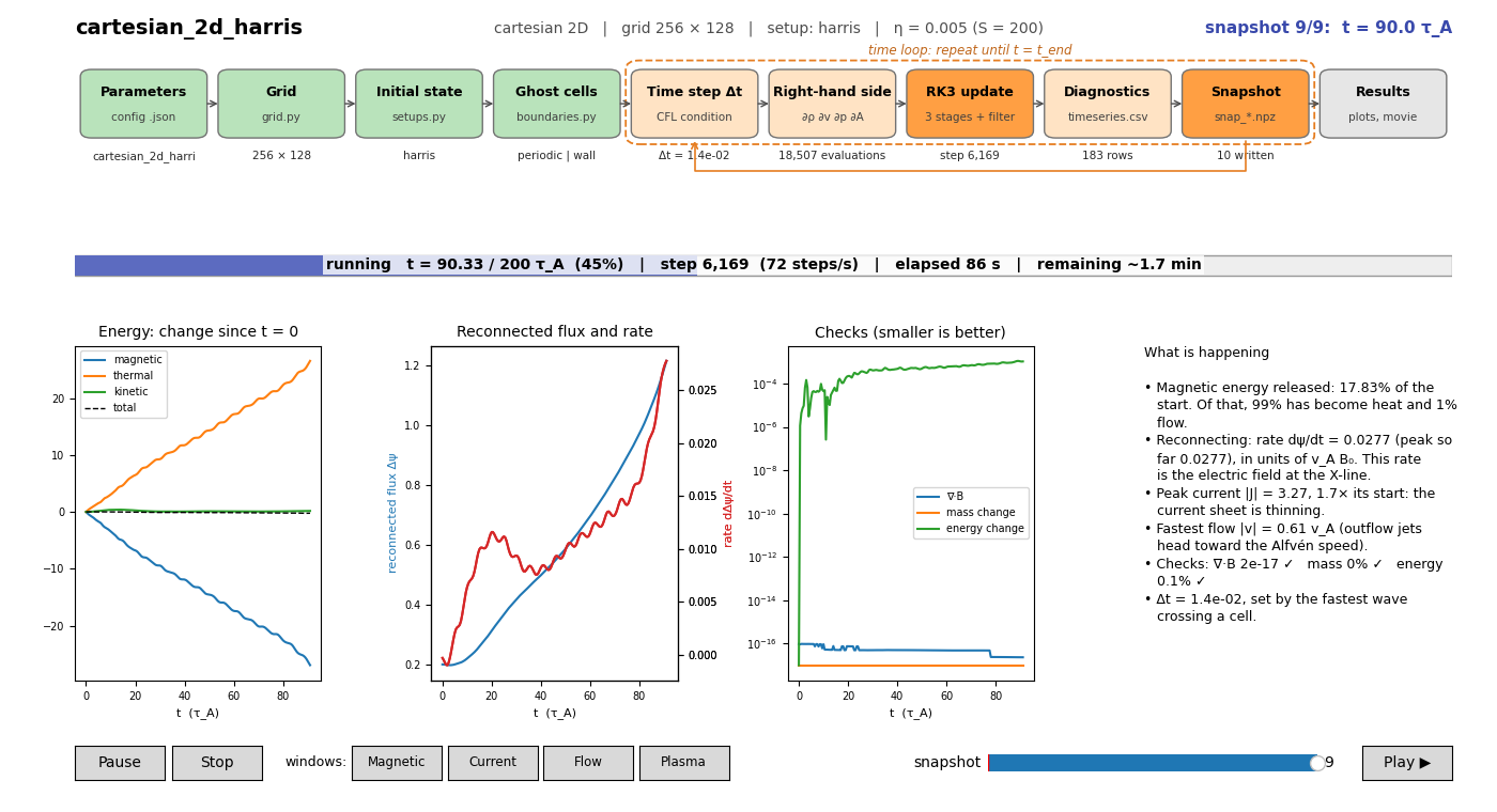
What the code does, in one picture

The config file sets up the grid, the initial state and the boundaries once. Then the time loop advances four equations again and again, writing diagnostics and snapshots on the way. Click a box to read how that step works. The Cartesian and Spherical pages show the chart for their 2D and 3D runs.

What the code solves

In code units (\(\mu_0 = 1\), lengths in \(L_0\), speeds in \(v_A\), times in \(\tau_A = L_0/v_A\); see dimensionless form), for density \(\rho\), velocity \(\mathbf{v}\), pressure \(p\) and vector potential \(\mathbf{A}\):

\[ \begin{aligned} \partial_t\rho &= -\nabla\cdot(\rho\mathbf{v}) \\ \partial_t\mathbf{v} &= -\nabla\tfrac{v^2}{2} + \mathbf{v}\times\boldsymbol{\omega} - \frac{\nabla p}{\rho} + \frac{\mathbf{J}\times\mathbf{B}}{\rho} + \mathbf{g} + \nu\left[\tfrac43\nabla(\nabla\cdot\mathbf{v}) - \nabla\times\boldsymbol{\omega}\right] \\ \partial_t p &= -\mathbf{v}\cdot\nabla p - \gamma p\nabla\cdot\mathbf{v} + (\gamma-1)\left[\eta J^2 + \rho\nu\left(\omega^2 + \tfrac43(\nabla\cdot\mathbf{v})^2\right)\right] \\ \partial_t\mathbf{A} &= \mathbf{v}\times\mathbf{B} - \eta\mathbf{J} \end{aligned} \]

with \(\mathbf{B} = \nabla\times\mathbf{A}\) (plus an optional uniform background field), \(\mathbf{J} = \nabla\times\mathbf{B}\) and vorticity \(\boldsymbol{\omega} = \nabla\times\mathbf{v}\). Discretizing the equations explains why they are written in this particular form.

What is in the zip file

File	Concept	Explained in
splmhd/grid.py	Cell-centred mesh, ghost cells, scale factors	Grid
splmhd/operators.py	grad, div, curl by central differences	Derivatives
splmhd/physics.py	Right-hand side of the equations	Right-hand side
splmhd/boundaries.py	Periodic, wall, fixed, open boundaries	Boundaries
splmhd/solver.py	RK3 time stepping, CFL, diagnostics, output	Time stepping
splmhd/setups.py	Initial conditions	Cartesian, Spherical
Start Lab.command, Start Lab.bat	Double-click to start (Mac, Windows)	Run it
lab.py	The lab: menu, parameter changes, live window, plots at the end	Run it
run.py	The solver's command line (the lab calls it)	Visualizing
tools/	Live monitor, plots, movies, 3D viewer, ParaView	Visualizing
configs/	Seven ready-made runs	the pages below

The example runs

Config	Physics	Run time*
cartesian_2d_alfven	Alfvén wave: a test against an exact solution	seconds
cartesian_2d_harris	Sweet–Parker reconnection of a Harris sheet	~4 min
cartesian_3d_harris	An X-line born in a patch that spreads along the current	~15 min
spherical_2d_dipole	A magnetosphere: driven reconnection at a dipole's null ring	~2 min
spherical_3d_dipole	The same in 3D, pushed on one patch of longitude	~10 min
spherical_2d_sheet, spherical_3d_sheet	Advanced: a current sheet in a gravitating corona	~5 / 15 min

*Measured on an Apple M3 laptop; expect 2–3 times longer on an older machine.

What this code is, and is not

splmhd is built for learning: second-order central differences, explicit time stepping, NumPy arrays, about 700 lines for the solver. It is accurate for smooth resistive flows like the ones here and checks itself (energy, mass, \(\nabla\cdot\mathbf{B}\)). It is not a shock-capturing research code and is about 100 times slower than compiled codes. When you need those, the same ideas carry over to community codes such as Athena++, PLUTO and the Pencil Code.