Discretizing the equations

A computer cannot store a continuous field such as \(\rho(x, y, z, t)\). It stores numbers at a finite set of points, and replaces every derivative with arithmetic on neighbouring numbers. This page builds the solver step by step:

1. choose variables and write the equations in a form that is easy to discretize;
2. lay out a grid, with ghost cells for the boundaries;
3. replace space derivatives with finite differences, in Cartesian or spherical coordinates;
4. assemble the right-hand side of every equation;
5. fill boundary cells;
6. advance in time without going unstable;
7. check the answer.

Every code excerpt below is quoted directly from the downloadable code, so the page and the code cannot disagree.

1. Choosing the variables

The code evolves \(\rho\), \(\mathbf{v}\), \(p\) and the vector potential \(\mathbf{A}\), not \(\mathbf{B}\).

Why \(\mathbf{A}\)? The equations require \(\nabla\cdot\mathbf{B} = 0\), but small numerical errors in an equation for \(\mathbf{B}\) can create \(\nabla\cdot\mathbf{B}\ne0\): fake magnetic monopoles that push the plasma along the field. If instead \(\mathbf{B} = \nabla\times\mathbf{A}\), then \(\nabla\cdot\mathbf{B} = 0\) holds automatically, and (as shown in section 3) it holds to round-off even on the grid. With the Weyl gauge the equation for \(\mathbf{A}\) is just Ohm's law, \(\partial_t\mathbf{A} = \mathbf{v}\times\mathbf{B} - \eta\mathbf{J}\) (derivation).

Why \(p\) and \(\mathbf{v}\) (not energy and momentum)? These "primitive" variables make the equations shortest and easiest to read. The price is that total energy is conserved only approximately (to about 0.5% in the example runs). Research codes for shocks use the conservative form instead.

Rewriting the vector terms. \((\mathbf{v}\cdot\nabla)\mathbf{v}\) and \(\nabla^2\mathbf{v}\) have awkward extra terms in curved coordinates. Two vector identities replace them with operators we need anyway:

\[ (\mathbf{v}\cdot\nabla)\mathbf{v} = \nabla\frac{v^2}{2} - \mathbf{v}\times(\nabla\times\mathbf{v}), \qquad \nabla^2\mathbf{v} = \nabla(\nabla\cdot\mathbf{v}) - \nabla\times(\nabla\times\mathbf{v}). \]

Then the whole system needs only four operators, grad, div, curl and cross/dot products, which work in any coordinate system once grad, div and curl are written for it.

The equations the code solves, on paper. In code units (\(\mu_0 = 1\)), with \(\mathbf{B} = \nabla\times\mathbf{A}\) (plus an optional uniform background field \(\mathbf{B}_{bg}\)), \(\mathbf{J} = \nabla\times\mathbf{B}\), vorticity \(\boldsymbol{\omega} = \nabla\times\mathbf{v}\) and temperature \(T = p/\rho\):

\[ \partial_t\rho = -\nabla\cdot(\rho\mathbf{v}) \tag{1} \]

\[ \begin{aligned} \partial_t\mathbf{v} = {}& -\nabla\tfrac{v^2}{2} + \mathbf{v}\times\boldsymbol{\omega} - \frac{\nabla p}{\rho} + \frac{\mathbf{J}\times\mathbf{B}}{\rho} + \mathbf{g} \\ & + \nu\left[\tfrac43\nabla(\nabla\cdot\mathbf{v}) - \nabla\times\boldsymbol{\omega}\right] \end{aligned} \tag{2} \]

\[ \begin{aligned} \partial_t p = {}& -\mathbf{v}\cdot\nabla p - \gamma p\,\nabla\cdot\mathbf{v} \\ & + (\gamma-1)\left[\eta\,|\mathbf{J}-\mathbf{J}_0|^2 + \rho\nu\left(\omega^2 + \tfrac43(\nabla\cdot\mathbf{v})^2\right) + \kappa\nabla^2T\right] \end{aligned} \tag{3} \]

\[ \partial_t\mathbf{A} = \mathbf{v}\times\mathbf{B} - \eta\,(\mathbf{J}-\mathbf{J}_0) \tag{4} \]

\(\mathbf{J}_0 = 0\) and \(\kappa = 0\) unless switched on in the config. Sections 2 and 3 build the grid and the differences; section 4 turns (1)–(4) into formulas for each cell, and section 6 advances them by \(\Delta t\).

The same four equations, discretized

Each of (1)–(4) is written out on the grid, every term labelled and linked to the section that explains it: continuity (1), momentum (2), pressure (3), induction (4). All of them together, every component written out and every abbreviation defined: the equation sheet. The order in which the code runs them: the flow charts.

2. The grid

The domain is divided into cells of size \(\Delta x_1\times\Delta x_2\times\Delta x_3\), and each variable is stored at the cell centre. Around the physical cells sit two layers of ghost cells on every side. They hold copies or mirror images set by the boundary conditions, so the same derivative formula works right up to the edge.

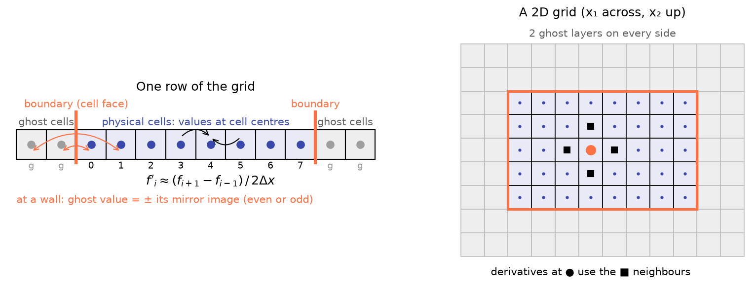
2D and 3D with the same code. A direction with a single cell is treated as invariant: every derivative along it is zero and it gets no ghost cells. A grid of \(256\times128\times1\) is therefore a 2D simulation in which every vector still has three components (sometimes called 2.5D). That is how a guide field \(B_z\), or an out-of-plane current \(J_z\), lives in a 2D run.

splmhd/grid.py (excerpt)

self.active = tuple(k > 1 for k in self.n)        # which directions vary
self.ng = tuple(NG if a else 0 for a in self.active)  # NG = 2 ghost layers
# cell centres, ghost cells included:
k = np.arange(-self.ng[i], self.n[i] + self.ng[i])
self.x.append(self.lo[i] + (k + 0.5) * self.d[i])

3. Derivatives on a grid

Central differences

Write the Taylor series of \(f\) about a cell centre \(x_i\), one cell either side:

\[ f_{i\pm1} = f_i \pm \Delta x\,f'_i + \frac{\Delta x^2}{2}f''_i \pm \frac{\Delta x^3}{6}f'''_i + \dots \]

Subtracting the two cancels every even term:

\[ \boxed{\;f'_i = \frac{f_{i+1} - f_{i-1}}{2\Delta x} - \frac{\Delta x^2}{6}f'''_i + \dots\;} \]

The error shrinks as \(\Delta x^2\): second-order accurate. Halving the cell size makes it four times smaller. In NumPy the whole array is differentiated in one line by shifting slices instead of looping over cells:

splmhd/operators.py

def deriv(f, grid, axis):
    """Central difference of f along grid direction `axis` (0, 1 or 2)."""
    out = np.zeros_like(f)
    if not grid.active[axis]:
        return out  # invariant direction: d/dx = 0
    ax = f.ndim - 3 + axis
    centre = [slice(None)] * f.ndim
    plus = [slice(None)] * f.ndim
    minus = [slice(None)] * f.ndim
    centre[ax], plus[ax], minus[ax] = slice(1, -1), slice(2, None), slice(None, -2)
    out[tuple(centre)] = (f[tuple(plus)] - f[tuple(minus)]) / (2.0 * grid.d[axis])
    return out

The difference operators D₁, D₂, D₃

Every derivative in the rest of this page is written with one of three operators. \(D_m\) is the central difference along grid direction \(m\): take whatever stands after it, look up its values in the two neighbouring cells along \(m\), subtract, and divide by the coordinate distance between those two cells, \(2\Delta x_m\):

\[ \begin{aligned} (D_1 f)_{i,j,k} &= \frac{f_{i+1,j,k} - f_{i-1,j,k}}{2\,\Delta x_1} \;\approx\; \frac{\partial f}{\partial x_1} &&\text{only } i \text{ changes} \\[6pt] (D_2 f)_{i,j,k} &= \frac{f_{i,j+1,k} - f_{i,j-1,k}}{2\,\Delta x_2} \;\approx\; \frac{\partial f}{\partial x_2} &&\text{only } j \text{ changes} \\[6pt] (D_3 f)_{i,j,k} &= \frac{f_{i,j,k+1} - f_{i,j,k-1}}{2\,\Delta x_3} \;\approx\; \frac{\partial f}{\partial x_3} &&\text{only } k \text{ changes} \end{aligned} \]

\(m\)	Cartesian \(x_m\), \(\Delta x_m\)	Spherical \(x_m\), \(\Delta x_m\)	Index that shifts	In the code
1	\(x\), \(\Delta x\)	\(r\), \(\Delta r\)	\(i\)	deriv(f, grid, 0)
2	\(y\), \(\Delta y\)	\(\theta\), \(\Delta\theta\) (an angle)	\(j\)	deriv(f, grid, 1)
3	\(z\), \(\Delta z\)	\(\phi\), \(\Delta\phi\) (an angle)	\(k\)	deriv(f, grid, 2)

Four rules make every formula below readable:

1. \(D_m\) differences everything that follows it, as one number per cell. \(D_1(h_2h_3\,\rho v_1)\) means: form the product \(h_2h_3\,\rho v_1\) in cell \(i+1\) and in cell \(i-1\), subtract, divide by \(2\Delta x_1\). It is not \(h_2h_3\,\rho\,D_1v_1\). Brackets show where the differenced quantity ends; in \(D_1K/h_1\) only \(K\) is differenced.
2. \(\Delta x_m\) is a step in the coordinate, not always a length. In spherical coordinates \(\Delta x_2 = \Delta\theta\) is an angle; the distance between the cells is \(h_2\,\Delta\theta = r\,\Delta\theta\). This is why a gradient component is \(D_m f/h_m\), and why the \(h_m\) appear everywhere below.
3. Along a direction with one cell, \(D_m = 0\). A 2D run has \(N_3 = 1\): nothing varies along \(x_3\) (2.5D), and deriv returns zero for that direction.
4. Two differences in a row reach two cells. \((D_1D_1f)_{i} = (f_{i+2} - 2f_i + f_{i-2})/(4\Delta x_1^2)\), and \(D_1D_2\) reaches the diagonal cells \((i\pm1, j\pm1)\). The current \(\mathbf J = \nabla_h\times(\nabla_h\times\mathbf A)\) and the Laplacian are of this kind.

A check with numbers. \(f = x^2\), \(\Delta x = 0.1\), at \(x_i = 1\): \((D_1f)_i = (1.1^2 - 0.9^2)/0.2 = (1.21 - 0.81)/0.2 = 2.00\), exactly \(f'(1) = 2\) (for a parabola \(f''' = 0\), so the error term vanishes). For \(f = x^3\): \((1.331 - 0.729)/0.2 = 3.01\) against \(f'(1) = 3\), an error of \(0.01 = \Delta x^2 f'''/6\), as the Taylor series predicts.

The derivative is valid one cell less far into the ghost layers than the field itself. Two ghost layers are therefore enough for two derivatives in a row, such as \(\mathbf{J} = \nabla\times(\nabla\times\mathbf{A})\).

Curvilinear coordinates: scale factors

In orthogonal coordinates \((x_1, x_2, x_3)\), a small step \(dx_m\) in direction \(m\) covers a physical distance \(h_m\,dx_m\). The scale factors \(h_m\) are all the geometry the code needs:

Geometry	\((x_1, x_2, x_3)\)	\((h_1, h_2, h_3)\)
Cartesian	\((x, y, z)\)	\((1, 1, 1)\)
Spherical	\((r, \theta, \phi)\)	\((1,\ r,\ r\sin\theta)\)

The general formulas for orthogonal coordinates are

\[ \nabla f = \left(\frac{\partial_1 f}{h_1}, \frac{\partial_2 f}{h_2}, \frac{\partial_3 f}{h_3}\right), \qquad \nabla\cdot\mathbf{F} = \frac{\partial_1(h_2h_3F_1) + \partial_2(h_3h_1F_2) + \partial_3(h_1h_2F_3)}{h_1h_2h_3}, \]

\[ (\nabla\times\mathbf{F})_1 = \frac{\partial_2(h_3F_3) - \partial_3(h_2F_2)}{h_2h_3} \quad\text{and cyclic permutations } (1\to2\to3\to1). \]

For spherical coordinates these give the familiar textbook results, for example

\[ \nabla\cdot\mathbf{F} = \frac{1}{r^2}\frac{\partial(r^2F_r)}{\partial r} + \frac{1}{r\sin\theta}\frac{\partial(\sin\theta F_\theta)}{\partial\theta} + \frac{1}{r\sin\theta}\frac{\partial F_\phi}{\partial\phi}. \]

On the grid, every \(\partial_m\) becomes \(D_m\). We write \(\nabla_h\), \(\nabla_h\cdot\) and \(\nabla_h\times\) for these discrete operators (the code's grad, div, curl). Note that the scale factors sit inside the difference: \(D_1(h_2h_3F_1)\) uses the products \(h_2h_3F_1\) in the neighbouring cells \(i\pm1\).

The code implements the general formulas once. Cartesian and spherical runs use exactly the same lines; only the arrays \(h_1, h_2, h_3\) differ:

splmhd/operators.py

def grad(f, g):
    h1, h2, h3 = g.h
    return np.array([deriv(f, g, 0) / h1, deriv(f, g, 1) / h2, deriv(f, g, 2) / h3])


def div(F, g):
    h1, h2, h3 = g.h
    return (deriv(h2 * h3 * F[0], g, 0)
            + deriv(h3 * h1 * F[1], g, 1)
            + deriv(h1 * h2 * F[2], g, 2)) / g.h123


def curl(F, g):
    h1, h2, h3 = g.h
    c1 = (deriv(h3 * F[2], g, 1) - deriv(h2 * F[1], g, 2)) / g.h23
    c2 = (deriv(h1 * F[0], g, 2) - deriv(h3 * F[2], g, 0)) / g.h31
    c3 = (deriv(h2 * F[1], g, 0) - deriv(h1 * F[0], g, 1)) / g.h12
    return np.array([c1, c2, c3])


def laplacian(f, g):
    return div(grad(f, g), g)

Why ∇·B stays exactly zero

Substituting the discrete curl into the discrete divergence gives

\[ h_1h_2h_3\,\nabla\cdot(\nabla\times\mathbf{A}) = D_1D_2(h_3A_3) - D_1D_3(h_2A_2) + D_2D_3(h_1A_1) - D_2D_1(h_3A_3) + D_3D_1(h_2A_2) - D_3D_2(h_1A_1). \]

Differences along different directions commute (\(D_1D_2 = D_2D_1\)): shifting in \(x_1\) then \(x_2\) reaches the same cells as shifting in \(x_2\) then \(x_1\). So the six terms cancel in pairs, and the discrete \(\nabla\cdot\mathbf{B}\) is zero up to round-off (about \(10^{-16}\) in the runs). The timeseries plot shows it.

4. Assembling the right-hand side

With the operators in place, each equation (1)–(4) becomes a formula for one cell. This section does it three ways for every equation: on paper, on the grid (with cell indices), and in the code. Every right-hand side is evaluated in all physical cells at once; the time step that uses it is in section 6.

All eight component equations together, on one sheet with every abbreviation defined, are in All the equations on one sheet; the order of the computation is chart 4.

Notation (the same on every part of this page)

Symbol	Meaning	In the code
\(u = (\rho, \mathbf{v}, p, \mathbf{A})\)	the state: everything the code evolves	state
\(i, j, k\)	cell index in \(x_1, x_2, x_3\). Physical cells \(i = 0\dots N_1-1\) (as in the figure of section 2); ghost cells \(i = -2, -1\) and \(N_1, N_1+1\)	array index \(i + 2\)
\(f_{i,j,k}\), \(f^n_{i,j,k}\)	the value of \(f\) at the centre of cell \((i,j,k)\) (at time \(t^n\))	f[..., i+2, j+2, k+2]
\(\Delta x_m\), \(h_m\)	cell width and scale factor in direction \(m\) (Cartesian: \(\Delta x, \Delta y, \Delta z\), \(h_m = 1\))	grid.d, grid.h
\(D_m\)	central difference along \(m\) (section 3)	deriv
\(\nabla_h, \nabla_h\cdot, \nabla_h\times\)	grad, div, curl built from \(D_m\)	grad, div, curl
\(L_\rho, L_{\mathbf v}, L_p, L_{\mathbf A}\)	the right-hand sides: \(du/dt = L(u)\)	drho, dv, dp, dA
\(\boldsymbol{\omega}\), \(K\)	vorticity \(\nabla\times\mathbf{v}\); kinetic energy per mass \(v^2/2\)	w, 0.5 * dot(v, v)
\(t^n\), \(\Delta t^n\), \(u^{(1)}, u^{(2)}\)	time and time step of step \(n\); Runge–Kutta stages	t, dt, u1, u2

In sections 6 and 7 a single direction is analysed, and there \(k\) is a wavenumber, not a cell index. A quantity written without indices inside a cell formula is taken in that same cell \((i,j,k)\).

The chain: what is computed from what, and where it is valid

The code stores only \(u\). Everything else is recomputed from it at each evaluation, in this order. A central difference reaches one cell to each side, so each step is valid one cell less far into the ghost layers (written for \(i\); the same holds for \(j\) and \(k\)):

#	Computed	Formula	Valid for	Code
0	ghost cells of \(u\)	boundary rules (section 5)	\(i = -2 \dots N_1+1\)	fill_ghosts
1	magnetic field	\(\mathbf{B} = \nabla_h\times\mathbf{A} + \mathbf{B}_{bg}\)	\(i = -1 \dots N_1\)	B = curl(A, grid) + aux["B_bg"]
2	current, vorticity, \(\nabla\cdot\mathbf v\)	\(\mathbf{J} = \nabla_h\times\mathbf{B}\), \(\boldsymbol{\omega} = \nabla_h\times\mathbf{v}\), \(\nabla_h\cdot\mathbf{v}\)	\(\mathbf J\): \(0\dots N_1-1\); \(\boldsymbol\omega\), \(\nabla_h\cdot\mathbf v\): \(-1\dots N_1\)	J = curl(B, grid), w = curl(v, grid), divv
3	right-hand sides	\(L_\rho, L_{\mathbf v}, L_p, L_{\mathbf A}\) below	\(i = 0\dots N_1-1\)	drho, dv, dp, dA
4	new state	one Runge–Kutta stage (section 6)	\(i = 0\dots N_1-1\), then back to step 0	stage

\(\mathbf{J} = \nabla_h\times(\nabla_h\times\mathbf{A})\) is two differences deep, which is why there are two ghost layers. In 2D Cartesian, for instance, it reaches two cells out: \((J_z)_{i,j} = -\big[(A_z)_{i+2,j} - 2(A_z)_{i,j} + (A_z)_{i-2,j}\big]/(4\Delta x^2) - \big[(A_z)_{i,j+2} - 2(A_z)_{i,j} + (A_z)_{i,j-2}\big]/(4\Delta y^2)\).

The building blocks

The four equations below use only these pieces. Each is a formula for one cell \((i,j,k)\), and each is explained in the section given on the right.

Piece	On the grid, in cell \((i,j,k)\)	Explained in
central difference \(D_m\)	\((D_1f)_{i,j,k} = \dfrac{f_{i+1,j,k} - f_{i-1,j,k}}{2\Delta x_1}\), and \(D_2\), \(D_3\) shift \(j\), \(k\)	§3 The difference operators
scale factors \(h_m\)	Cartesian \((1, 1, 1)\); spherical \((1,\ r_i,\ r_i\sin\theta_j)\)	§3 Scale factors
magnetic field \(\mathbf B\)	\(B_1 = \dfrac{D_2(h_3A_3) - D_3(h_2A_2)}{h_2h_3} + B_{bg,1}\), and cyclic \((1\to2\to3\to1)\)	§1 Why A, §3 curl, ∇·B = 0
current \(\mathbf J\)	\(J_1 = \dfrac{D_2(h_3B_3) - D_3(h_2B_2)}{h_2h_3}\), and cyclic	the chain (why two ghost layers)
vorticity \(\boldsymbol\omega\)	\(\omega_1 = \dfrac{D_2(h_3v_3) - D_3(h_2v_2)}{h_2h_3}\), and cyclic	§1 vector identities
divergence \(\nabla_h\cdot\mathbf v\)	\(\dfrac{D_1(h_2h_3v_1) + D_2(h_3h_1v_2) + D_3(h_1h_2v_3)}{h_1h_2h_3}\)	§3
Laplacian \(\nabla_h\cdot\nabla_h f\)	\(\dfrac{1}{h_1h_2h_3}\displaystyle\sum_{m=1}^3 D_m\!\left(\frac{h_1h_2h_3}{h_m^2}\,D_mf\right)\) (the divergence of the gradient)	§3
filter \(\delta^4_m\)	\((\delta^4_1f)_{i,j,k} = f_{i+2,j,k} - 4f_{i+1,j,k} + 6f_{i,j,k} - 4f_{i-1,j,k} + f_{i-2,j,k}\)	§7 Filter
cells beyond the edge	\(f_{-2}, f_{-1}, f_{N}, f_{N+1}\): set by the boundary rules before every evaluation	§5 Boundaries

Everything without an index below is taken in cell \((i,j,k)\): for example \(h_1\) means \((h_1)_{i,j,k}\) and \(\rho\) means \(\rho_{i,j,k}\). The only places that reach other cells are the \(D_m\) (one cell each way) and the \(\delta^4_m\) (two cells each way). Each equation is shown in three forms: (I) on paper, (II) on the grid with every term labelled, and (III) one term fully written out with its indices.

Continuity, equation (1)

(I) On paper: \(\partial_t\rho = -\nabla\cdot(\rho\mathbf v)\).

(II) On the grid:

\[ \begin{aligned} \frac{d\rho_{i,j,k}}{dt} = (L_\rho)_{i,j,k} = {}& \underbrace{-\frac{D_1(h_2h_3\,\rho v_1) + D_2(h_3h_1\,\rho v_2) + D_3(h_1h_2\,\rho v_3)}{h_1h_2h_3}}_{\text{(a)}} \\[6pt] & \underbrace{-\ \frac{\sigma}{\Delta t^n}\sum_{m=1}^3\delta^4_m(\rho - \rho_0)}_{\text{(b)}} \ \underbrace{+\ \epsilon\,\nabla_h\cdot\nabla_h(\rho - \rho_0)}_{\text{(c)}} \end{aligned} \]

Term	Meaning	Explained in
(a)	mass flowing in from the neighbours minus mass flowing out: \(-\nabla\cdot(\rho\mathbf v)\)	§3, spherical form on the equation sheet
(b)	numerical filter, damps zig-zags from cell to cell (\(\sigma\) = config filter)	§7
(c)	optional numerical diffusion of the deviation from the initial state, \(\epsilon\) = config diffusion, off by default	the code

(III) Term (a) written out, the first of its three differences:

\[ \frac{D_1(h_2h_3\,\rho v_1)}{h_1h_2h_3}\bigg|_{i,j,k} = \frac{(h_2h_3\,\rho v_1)_{i+1,j,k} - (h_2h_3\,\rho v_1)_{i-1,j,k}}{2\Delta x_1\,(h_1h_2h_3)_{i,j,k}} \;\overset{\text{Cartesian}}{=}\; \frac{(\rho v_x)_{i+1,j,k} - (\rho v_x)_{i-1,j,k}}{2\Delta x}. \]

Momentum, equation (2)

(I) On paper: \(\partial_t\mathbf v = -\nabla\tfrac{v^2}{2} + \mathbf v\times\boldsymbol\omega - \dfrac{\nabla p}{\rho} + \dfrac{\mathbf J\times\mathbf B}{\rho} + \mathbf g + \nu\big[\tfrac43\nabla(\nabla\cdot\mathbf v) - \nabla\times\boldsymbol\omega\big]\).

(II) On the grid, component 1 (components 2 and 3 follow by the cyclic change \(1\to2\to3\to1\)), with \(K = \tfrac12(v_1^2 + v_2^2 + v_3^2)\):

\[ \begin{aligned} \frac{d(v_1)_{i,j,k}}{dt} = (L_{v_1})_{i,j,k} = {}& \underbrace{-\frac{D_1K}{h_1}}_{\text{(a)}} \ \underbrace{+\ \big(v_2\,\omega_3 - v_3\,\omega_2\big)}_{\text{(b)}} \ \underbrace{-\ \frac{D_1p}{h_1\,\rho}}_{\text{(c)}} \ \underbrace{+\ \frac{J_2B_3 - J_3B_2}{\rho}}_{\text{(d)}} \ \underbrace{+\ g_1}_{\text{(e)}} \\[6pt] & \underbrace{+\ \nu\left[\frac43\,\frac{D_1(\nabla_h\cdot\mathbf v)}{h_1} - \frac{D_2(h_3\,\omega_3) - D_3(h_2\,\omega_2)}{h_2h_3}\right]}_{\text{(f)}} \ \underbrace{-\ \frac{\sigma}{\Delta t^n}\sum_{m=1}^3\delta^4_m v_1}_{\text{(g)}} \end{aligned} \]

Term	Meaning	Explained in
(a) + (b)	the advection \(-(\mathbf v\cdot\nabla)\mathbf v\), rewritten as \(-\nabla K + \mathbf v\times\boldsymbol\omega\) so it is the same in any coordinates	§1
(c)	pressure gradient force per unit mass	§3 grad
(d)	Lorentz force \(\mathbf J\times\mathbf B\): the magnetic tension and pressure that drive the reconnection jets; a product in the same cell	the chain (\(\mathbf B\), \(\mathbf J\))
(e)	gravity, only in the spherical runs	Spherical
(f)	viscosity, \(\nu\big[\nabla^2\mathbf v + \tfrac13\nabla(\nabla\cdot\mathbf v)\big]\), with \(\nabla^2\mathbf v = \nabla(\nabla\cdot\mathbf v) - \nabla\times\boldsymbol\omega\) so it is the same in any coordinates	§1
(g)	numerical filter	§7

(III) Term (d) written out, in 2D Cartesian (\(\partial_z = 0\)), where \(\mathbf B\) and \(\mathbf J\) come from \(\mathbf A\) through the chain:

\[ \begin{aligned} &\left(\frac{J_yB_z - J_zB_y}{\rho}\right)_{i,j} \quad\text{with, for example,} \\[6pt] (B_y)_{i,j} &= -\frac{(A_z)_{i+1,j} - (A_z)_{i-1,j}}{2\Delta x}, \\[6pt] (J_z)_{i,j} &= \frac{(B_y)_{i+1,j} - (B_y)_{i-1,j}}{2\Delta x} - \frac{(B_x)_{i,j+1} - (B_x)_{i,j-1}}{2\Delta y}. \end{aligned} \]

The other components, term by term: the equation sheet.

Pressure, equation (3)

(I) On paper: \(\partial_t p = -\mathbf v\cdot\nabla p - \gamma p\,\nabla\cdot\mathbf v + (\gamma-1)\big[\eta|\mathbf J-\mathbf J_0|^2 + \rho\nu\big(\omega^2 + \tfrac43(\nabla\cdot\mathbf v)^2\big) + \kappa\nabla^2T\big]\).

(II) On the grid:

\[ \begin{aligned} \frac{dp_{i,j,k}}{dt} = (L_p)_{i,j,k} = {}& \underbrace{-\left(\frac{v_1\,D_1p}{h_1} + \frac{v_2\,D_2p}{h_2} + \frac{v_3\,D_3p}{h_3}\right)}_{\text{(a)}} \ \underbrace{-\ \gamma\,p\,\nabla_h\cdot\mathbf v}_{\text{(b)}} \\[6pt] & + (\gamma - 1)\Big[\underbrace{\eta\,|\mathbf J - \mathbf J_0|^2}_{\text{(c)}} + \underbrace{\rho\nu\big(\omega_1^2 + \omega_2^2 + \omega_3^2 + \tfrac43(\nabla_h\cdot\mathbf v)^2\big)}_{\text{(d)}} + \underbrace{\kappa\,\nabla_h\cdot\nabla_h T}_{\text{(e)}}\Big] \\[6pt] & \underbrace{-\ \frac{\sigma}{\Delta t^n}\sum_{m=1}^3\delta^4_m(p - p_0)}_{\text{(f)}} \ \underbrace{+\ \epsilon\,\nabla_h\cdot\nabla_h(p - p_0)}_{\text{(g)}}, \qquad T = p/\rho \end{aligned} \]

Term	Meaning	Explained in
(a)	the pressure carried along by the flow	§3 grad
(b)	compression heats, expansion cools (\(\gamma = 5/3\))	§3 div
(c)	ohmic heating: where the magnetic energy released by reconnection becomes heat (\(\mathbf J_0 = 0\) unless sustain_equilibrium)	the code
(d)	viscous heating: \(\rho\nu[\omega^2 + \tfrac43(\nabla_h\cdot\mathbf v)^2]\) captures shear and compressional heating in scalar curvilinear form	§1
(e)	heat conduction, off unless kappa > 0	building blocks (Laplacian)
(f), (g)	numerical filter and optional diffusion, as in (1)	§7

(III) Term (a) written out, Cartesian, the \(x\) part: \(\left(\dfrac{v_1D_1p}{h_1}\right)_{i,j,k} = (v_x)_{i,j,k}\,\dfrac{p_{i+1,j,k} - p_{i-1,j,k}}{2\Delta x}\): the velocity in the cell times the pressure difference across it.

Induction, equation (4)

(I) On paper: \(\partial_t\mathbf A = \mathbf v\times\mathbf B - \eta\,(\mathbf J - \mathbf J_0)\).

(II) On the grid, component 1 (and cyclic):

\[ \frac{d(A_1)_{i,j,k}}{dt} = (L_{A_1})_{i,j,k} = \underbrace{v_2B_3 - v_3B_2}_{\text{(a)}} \ \underbrace{-\ \eta\,\big(J_1 - J_{0,1}\big)}_{\text{(b)}} \]

Term	Meaning	Explained in
(a)	\(\mathbf v\times\mathbf B = -\mathbf E\) of ideal MHD: the field is carried with the plasma	the chain (\(\mathbf B\))
(b)	resistivity: the only term that lets field lines slip through the plasma, so the only cause of reconnection (no filter on \(\mathbf A\))	§7, Cartesian runs

(III) Written out. There is nothing more to expand: the update of \(\mathbf A\) is pointwise, and all its differences are inside \(\mathbf B\) and \(\mathbf J\). In 2D at the X-line, where \(\mathbf v = 0\) and \(\mathbf B = 0\), it is just \(\big(dA_z/dt\big)_{i,j} = -\eta\,(J_z)_{i,j}\): the reconnection rate.

From the four equations to the next time step

(II) gives \(du_{i,j,k}/dt = L_{i,j,k}(u)\) for all eight numbers in every cell (\(\rho\), three of \(\mathbf v\), \(p\), three of \(\mathbf A\)). The step from \(t^n\) to \(t^{n+1} = t^n + \Delta t^n\) evaluates all of (1)–(4) three times and blends (§6 RK3), with \(\Delta t^n\) from the CFL condition and the ghost cells refilled (§5) before each evaluation. For the density in one cell, the first of the three stages is

\[ \rho^{(1)}_{i,j,k} = \rho^n_{i,j,k} + \Delta t^n\,(L_\rho)_{i,j,k}(u^n) = \rho^n_{i,j,k} - \Delta t^n\left[\frac{(\rho v_x)^n_{i+1,j,k} - (\rho v_x)^n_{i-1,j,k}}{2\Delta x} + \dots\right] + \dots \]

All of it in code

The function below is equations (1)–(4) as the chain computes them. Match it line by line with the formulas above:

Formula	Line in rhs
\(\mathbf{B} = \nabla_h\times\mathbf{A} + \mathbf{B}_{bg}\), \(\mathbf{J} = \nabla_h\times\mathbf{B}\), \(\boldsymbol\omega = \nabla_h\times\mathbf{v}\)	B = curl(A, grid) + aux["B_bg"], J = curl(B, grid), w = curl(v, grid)
\(L_\rho\) (1)	drho = -div(rho * v, grid)
\(L_{\mathbf v}\) (2)	dv = (-grad(0.5 * dot(v, v), grid) + cross(v, w) - grad(p, grid) / rho + cross(J, B) / rho + nu * (...))
\(L_p\) (3)	dp = -dot(v, grad(p, grid)) - gam * p * divv + (gam - 1.0) * heating
\(L_{\mathbf A}\) (4)	dA = cross(v, B) - eta * Jr, with Jr \(= \mathbf J - \mathbf J_0\)
filter, section 7	drho -= rate * fourth_difference(rho - aux["rho0"], grid), etc.

splmhd/physics.py

def rhs(state, grid, par, aux):
    """Time derivatives of (rho, v, p, A) on the physical cells."""
    rho, v, p, A = state["rho"], state["v"], state["p"], state["A"]
    gam, nu, kappa, D = par["gamma"], par["nu"], par["kappa"], par["diffusion"]
    eta = aux["eta"]  # resistivity: a number or an array (localized resistivity)

    B = curl(A, grid) + aux["B_bg"]
    J = curl(B, grid)               # Ampere's law with mu0 = 1
    w = curl(v, grid)               # vorticity
    divv = div(v, grid)

    # Continuity
    drho = -div(rho * v, grid)

    # Momentum: (v.grad)v = grad(v^2/2) - v x w, valid in any coordinates
    dv = (-grad(0.5 * dot(v, v), grid) + cross(v, w)
          - grad(p, grid) / rho + cross(J, B) / rho
          + nu * (4.0 / 3.0 * grad(divv, grid) - curl(w, grid)))
    if aux["gravity"] is not None:
        dv += aux["gravity"]

    Jr = J - aux["J0"]  # resistive current (J0 = 0 unless the equilibrium is sustained)

    # Pressure (internal energy) with ohmic and viscous heating
    heating = eta * dot(Jr, Jr) + rho * nu * (dot(w, w) + 4.0 / 3.0 * divv**2)
    dp = -dot(v, grad(p, grid)) - gam * p * divv + (gam - 1.0) * heating
    if kappa > 0:
        dp += (gam - 1.0) * kappa * laplacian(p / rho, grid)

    # Induction, written for the vector potential: dA/dt = -E = v x B - eta J
    dA = cross(v, B) - eta * Jr

    if D > 0:
        drho += D * laplacian(rho - aux["rho0"], grid)
        dp += D * laplacian(p - aux["p0"], grid)

    rate = aux.get("filter_rate", 0.0)  # sigma / dt, set by the time stepper
    if rate > 0:
        drho -= rate * fourth_difference(rho - aux["rho0"], grid)
        dp -= rate * fourth_difference(p - aux["p0"], grid)
        dv -= rate * fourth_difference(v, grid)

    return {"rho": drho, "v": dv, "p": dp, "A": dA}

Three details:

• J0 is zero by default. With sustain_equilibrium switched on (used for the spherical runs), an applied field \(\mathbf{E}_0 = \eta\mathbf{J}_0\) stops the initial current sheet from slowly diffusing away, so only the perturbation reconnects.
• eta may be a number or an array \(\eta_{i,j,k}\): a localized resistivity around the X-line is a one-line change.
• diffusion and filter_rate are numerical terms, explained in section 7.

5. Boundary conditions

Before every evaluation of the right-hand side, the ghost cells are filled. Four types are available, and each side of each direction gets its own. The animation shows, for each type, what goes into the two ghost cells on each side (orange) given the interior values (blue); it was made with the code's own fill_ghosts.

Jump to:PeriodicWallFixedOpenspeed 0.5×0.75×1×1.5×

Type	\(\rho, p\)	Velocity	Vector potential \(\mathbf{A}\)	Use
periodic	wrap around	wrap around	wrap around	Directions with no edge (x along a sheet)
wall	mirror (even)	normal component odd (zero at the wall), tangential even	held at its initial value	Perfectly conducting, free-slip wall
fixed	held at initial value	all components odd (zero at the boundary)	held at initial value	Line-tied boundary of a stratified atmosphere
open	copy of the edge cell	copy of the edge cell	linear extrapolation	Outflow (approximate)

Even and odd mirrors. The ghost cells of a wall hold the mirror image of the cells just inside. A mirror leaves a scalar (\(\rho, p\)) and the part of a vector along the wall unchanged, but turns the part pointing into the wall around: so \(\rho\), \(p\), \(v_t\) are even (\(f_{\text{ghost}} = +f_{\text{mirror}}\)) and \(v_n\) is odd (\(f_{\text{ghost}} = -f_{\text{mirror}}\)). The wall sits on a cell face, halfway between a cell and its mirror, so the value at the wall is their average and the slope across it is their difference. Odd makes the value zero: no plasma goes through, which is how the normal velocity is made to vanish. Even makes the slope zero: no pressure force through the wall and no viscous drag along it (free slip). A fixed boundary makes every velocity component odd, so the plasma cannot slide either (no slip). Holding \(\mathbf{A}\) fixed makes \(\partial_t\mathbf{A} = -\mathbf{E} = 0\) there: no tangential electric field, no flux crossing the wall, as for a perfect conductor.

splmhd/boundaries.py

def fill_ghosts(state, grid, bc, ref):
    """Fill the ghost cells of every field in `state` in place.

    bc[axis] = (lower_type, upper_type); ref = the initial state (for 'wall'/'fixed').
    """
    for axis in range(3):
        if not grid.active[axis]:
            continue
        for side in (0, 1):
            kind = bc[axis][side]
            if kind == "periodic":
                if side == 0:
                    for f in state.values():
                        _periodic(f, axis)
                continue
            for name in ("rho", "p"):
                if kind == "fixed":
                    _restore(state[name], ref[name], axis, side)
                elif kind == "wall":
                    _parity(state[name], axis, side, +1)
                else:  # open
                    _copy_edge(state[name], axis, side)
            v = state["v"]
            for c in range(3):
                if kind == "wall":
                    _parity(v[c], axis, side, -1 if c == axis else +1)
                elif kind == "fixed":
                    _parity(v[c], axis, side, -1)
                else:  # open
                    _copy_edge(v[c], axis, side)
            if kind in ("wall", "fixed"):
                _restore(state["A"], ref["A"], axis, side)
            else:
                _extrapolate(state["A"], axis, side)

6. Time stepping

What a time step has to achieve

Section 4 gives, in every cell, only how fast the state is changing at this instant: \(L(u)\). A time step has to turn that into the state a time \(\Delta t\) later, and the whole run is that step repeated until \(t_{\text{end}}\). Two questions decide whether it works:

1. How big may \(\Delta t\) be? If it is too big, errors do not just get larger, they grow without bound and the run blows up. The answer is the CFL condition, below.
2. How should \(L\) be used within the step? \(L\) changes during the step, so using only its value at the start (one Euler step) is inaccurate and, for waves, unstable at any \(\Delta t\). The answer is RK3: sample \(L\) three times and blend.

The video shows both on the simplest wave there is, a pulse carried at speed \(c\) and computed with the same central difference and RK3 as splmhd: a step that is too big blows up, the code's step does not, Euler fails where RK3 works, then the two mins of the code's formula on a real grid, and the loop.

Jump to:1. The goal2. Signal & grid3. Δt too big4. With CFL5. min min6. RK3 stages7. Why RK38. The loopspeed 0.5×0.75×1×1.5×

Method of lines

After discretizing space, every cell value \(u_{i,j,k}\) obeys an ordinary differential equation, \(du_{i,j,k}/dt = L_{i,j,k}(u)\), where \(L\) is the right-hand side of section 4. Any ODE solver could advance it. The choice matters because of stability.

Why not the simplest method?

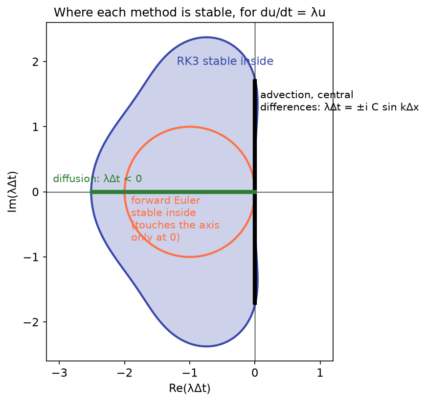
Forward Euler, \(u^{n+1} = u^n + \Delta t\,L(u^n)\), is unstable with central differences. Try it on the advection equation \(\partial_tu + c\,\partial_xu = 0\) with a wave \(u_i = \hat u\,e^{ikx_i}\). The central difference gives \(L = -i\,(c/\Delta x)\sin(k\Delta x)\,u\), so each step multiplies the wave by

\[ G = 1 - i\,\frac{c\Delta t}{\Delta x}\sin(k\Delta x), \qquad |G|^2 = 1 + \left(\frac{c\Delta t}{\Delta x}\right)^2\sin^2(k\Delta x) > 1 . \]

Every wave grows a little at every step, for any \(\Delta t\). Central differences of advection produce purely imaginary rates (pure oscillation, no damping), and forward Euler's stability region does not contain the imaginary axis.

Third-order Runge–Kutta

The code uses the strong-stability-preserving third-order Runge–Kutta method (SSP-RK3, Shu & Osher 1988). Its stability region contains a stretch of the imaginary axis, \(|\lambda\Delta t|\le\sqrt3\), and of the negative real axis down to about \(-2.5\), so it handles both waves and diffusion:

One step from \(t^n\) to \(t^{n+1} = t^n + \Delta t^n\) takes three stages. Each is applied to every physical cell \((i,j,k)\), and to all four variables \(\rho, \mathbf{v}, p, \mathbf{A}\) together:

\[ \begin{aligned} u^{(1)}_{i,j,k} &= u^n_{i,j,k} + \Delta t^n\,L_{i,j,k}(u^n) \\ u^{(2)}_{i,j,k} &= \tfrac34\,u^n_{i,j,k} + \tfrac14\Big[u^{(1)}_{i,j,k} + \Delta t^n\,L_{i,j,k}\big(u^{(1)}\big)\Big] \\ u^{n+1}_{i,j,k} &= \tfrac13\,u^n_{i,j,k} + \tfrac23\Big[u^{(2)}_{i,j,k} + \Delta t^n\,L_{i,j,k}\big(u^{(2)}\big)\Big] \end{aligned} \]

After each stage the code applies the floors, \(\rho_{i,j,k} \leftarrow \max(\rho_{i,j,k}, \rho_{\text{floor}})\) and the same for \(p\), and fills the ghost cells of the new state (section 5), because the next \(L\) needs them. For example, the density in one cell after the first stage is

\[ \rho^{(1)}_{i,j,k} = \rho^n_{i,j,k} - \Delta t^n \left[\frac{(\rho v_x)^n_{i+1,j,k} - (\rho v_x)^n_{i-1,j,k}}{2\Delta x} + \dots\right], \]

and \(\mathbf{A}\) moves by \(\Delta t^n(\mathbf v\times\mathbf B - \eta\mathbf J)\) in each cell.

What the three stages achieve. Write \(k_1 = L(u^n)\), \(k_2 = L(u^{(1)})\), \(k_3 = L(u^{(2)})\) for the three slopes. Putting the stages into each other gives

\[ u^{(1)} = u^n + \Delta t\,k_1, \qquad u^{(2)} = u^n + \tfrac{\Delta t}{2}\cdot\frac{k_1 + k_2}{2}, \qquad u^{n+1} = u^n + \Delta t\left(\tfrac16k_1 + \tfrac16k_2 + \tfrac23k_3\right). \]

• Stage 1 is a trial Euler step to the end of the step. It is not kept; its job is to give a slope there, \(k_2\).
• Stage 2 averages the start and end slopes and goes half a step: \(u^{(2)}\) estimates the state at \(t^n + \Delta t/2\), and gives the slope in the middle, \(k_3\).
• Stage 3 takes the real step with the average slope over the step from start, end and middle, weighted \(\tfrac16, \tfrac16, \tfrac23\), Simpson's rule.

The result is accurate to third order (the error per unit time shrinks as \(\Delta t^3\), against \(\Delta t\) for Euler), and, the reason the code needs it, it is stable for waves up to \(C = \sqrt3\). In the video's example one RK3 step lands 13 times closer to the exact answer than one Euler step of the same size. In the code, all three stages are one function, stage(base, current, a, b), which computes a * base + b * (current + dt * L(current)) with \((a, b) = (0, 1)\), \((\tfrac34, \tfrac14)\), \((\tfrac13, \tfrac23)\):

splmhd/solver.py

def rk3_step(state, grid, bc, par, aux, ref, dt, floors):
    """Strong-stability-preserving 3rd-order Runge-Kutta (Shu & Osher 1988).

    u1      = u + dt L(u)
    u2      = 3/4 u + 1/4 (u1 + dt L(u1))
    u(n+1)  = 1/3 u + 2/3 (u2 + dt L(u2))
    """
    I = {k: (grid.inner_vec if state[k].ndim == 4 else grid.inner) for k in state}
    aux["filter_rate"] = par["filter"] / dt

    def stage(base, current, a, b):
        L = rhs(current, grid, par, aux)
        new = {k: v.copy() for k, v in current.items()}
        for k in new:
            new[k][I[k]] = a * base[k][I[k]] + b * (current[k][I[k]] + dt * L[k][I[k]])
        np.maximum(new["rho"], floors[0], out=new["rho"])
        np.maximum(new["p"], floors[1], out=new["p"])
        boundaries.fill_ghosts(new, grid, bc, ref)
        return new

    u1 = stage(state, state, 0.0, 1.0)
    u2 = stage(state, u1, 0.75, 0.25)
    return stage(state, u2, 1.0 / 3.0, 2.0 / 3.0)

The CFL condition

What it achieves. A cell's new value is computed from its neighbours only, so a signal must not travel further in one step than those neighbours: otherwise the formula cannot see where the signal comes from, and computes the wrong thing, and the error grows from step to step. In terms of section 6, the eigenvalues must stay inside the stability region. So the time step must be small enough that the fastest signal crosses less than about one cell per step (Courant, Friedrichs and Lewy, 1928). In MHD the fastest signal is the fast magnetosonic wave, \(c_f = \sqrt{c_s^2 + v_A^2}\) with \(c_s^2 = \gamma p/\rho\), carried by the flow. Diffusion adds a second limit, because a diffusive rate grows as \(1/\Delta x^2\):

\[ \Delta t^n = C\,\min\!\left[\ \min_{\text{cells},\ m}\frac{h_m\Delta x_m}{|\mathbf{v}| + c_f},\ \ \frac{\Delta x_{\min}^2}{2\,d\,\max(\eta,\nu)}\ \right], \]

where \(d\) is the number of dimensions and \(C\approx0.4\) is the CFL number, a safety factor. Read it from the inside out:

1. In each cell and each direction \(m\): \(h_m\Delta x_m/(|\mathbf v| + c_f)\) is the time the fastest signal in that cell needs to cross it. The inner min over directions takes the narrowest side of the cell; over cells it takes the cell where this time is shortest. One cell decides for the whole grid, because all cells take the same step.
2. Diffusion: \(\Delta x_{\min}^2/(2d\max(\eta,\nu))\) is the time over which resistivity or viscosity smooths a bump one cell wide; an explicit step longer than that overshoots and oscillates.
3. The outer min takes the stricter of the two limits, and \(C\) leaves a margin. RK3 alone would allow \(C = \sqrt3\) for one wave in 1D; 0.4 covers waves crossing in two or three directions at once, speeds that change during the step, and the filter.

On the 14 × 8 demonstration grid of the video: the shortest crossing time is 0.382, the diffusion limit is 50, so \(\Delta t = 0.4 \times 0.382 = 0.153\). The wave limit almost always wins; diffusion only matters for very fine grids or large \(\eta\). Because the speeds change as the run goes, \(\Delta t\) is recomputed at the start of every step.

splmhd/solver.py

def timestep(state, grid, par, aux, cfl):
    """Largest stable dt: waves must not cross a cell, diffusion must not overshoot."""
    I = grid.inner
    rho, p = state["rho"][I], state["p"][I]
    B = (curl(state["A"], grid) + aux["B_bg"])[grid.inner_vec]
    v = state["v"][grid.inner_vec]
    cfast = np.sqrt((par["gamma"] * p + (B**2).sum(0)) / rho)  # fast magnetosonic speed
    vmax = np.sqrt((v**2).sum(0)) + cfast
    widths = grid.spacing_fields()
    dt_wave = min((w / vmax).min() for w in widths)

    eta_max = np.max(aux["eta"])
    diff = max(eta_max, par["nu"], par["diffusion"],
               (par["gamma"] - 1) * par["kappa"] / rho.min())
    dx_min = grid.min_spacing()
    dt_diff = dx_min**2 / (2 * grid.dims * diff) if diff > 0 else np.inf
    return cfl * min(dt_wave, dt_diff)

Why spherical runs take more steps

The physical cell width in \(\theta\) is \(r\,\Delta\theta\), smallest at the inner radius, and in \(\phi\) it is \(r\sin\theta\,\Delta\phi\), smaller still near the poles. The smallest cell sets the time step for the whole grid. This is also why the spherical domain stops short of the poles: there \(\sin\theta\to0\), the cells shrink to nothing, and \(1/(r\sin\theta)\) in the operators blows up.

7. Grid noise and the filter

Central differences have no built-in damping. Look at the shortest wave the grid can hold, the one-cell zig-zag \(+1, -1, +1, \ldots\) (\(k\Delta x = \pi\)): its central difference is \((f_{i+1} - f_{i-1})/2\Delta x = 0\). The scheme cannot even see it, so nothing stops it from growing where the solution is barely resolved.

This happened during the testing of this code. A Harris-sheet run at \(\eta = 5\times10^{-3}\) ran smoothly for 96 Alfvén times. Then the Sweet–Parker sheet thinned to about two cells, zig-zag noise appeared at the X-line, the density hit zero, and the run collapsed in less than one time unit.

The cure is a weak fourth-difference filter, added to the equations for \(\rho\), \(\mathbf{v}\) and \(p\):

\[ (L_f)_{i,j,k} \;\leftarrow\; (L_f)_{i,j,k} - \frac{\sigma}{\Delta t^n}\Big[\big(f_{i+2} - 4f_{i+1} + 6f_i - 4f_{i-1} + f_{i-2}\big) + \big(\text{same along } j\big) + \big(\text{same along } k\big)\Big], \]

with \(f = \rho - \rho_0\), \(p - p_0\) or each component of \(\mathbf v\) (only the indices that change are written).

For a wave \(e^{ikx}\) the bracket is \(16\sin^4(k\Delta x/2)\,f\). So each step removes a fraction \(16\sigma\) of the zig-zag mode (16% for \(\sigma = 0.01\)), but only about \(10^{-4}\sigma\) of a feature 20 cells wide. It is not applied to \(\mathbf{A}\), so reconnection in the code is caused by \(\eta\) and nothing else.

splmhd/operators.py

def fourth_difference(f, grid):
    """Sum over active directions of f[i+2] - 4f[i+1] + 6f[i] - 4f[i-1] + f[i-2] (grid units)."""
    out = np.zeros_like(f)
    for axis in range(3):
        if not grid.active[axis]:
            continue
        ax = f.ndim - 3 + axis
        n = f.shape[ax]

        def s(a, b):
            idx = [slice(None)] * f.ndim
            idx[ax] = slice(a, n + b if n + b != n else None)
            return tuple(idx)

        out[s(2, -2)] += f[s(4, 0)] - 4 * f[s(3, -1)] + 6 * f[s(2, -2)] - 4 * f[s(1, -3)] + f[s(0, -4)]
    return out

Two last safety nets: floors keep \(\rho\) and \(p\) above tiny positive values, and the run stops with advice if the time step collapses or a value becomes NaN.

8. Checking the answer

A simulation is only useful if you know how wrong it is. splmhd checks itself in three ways.

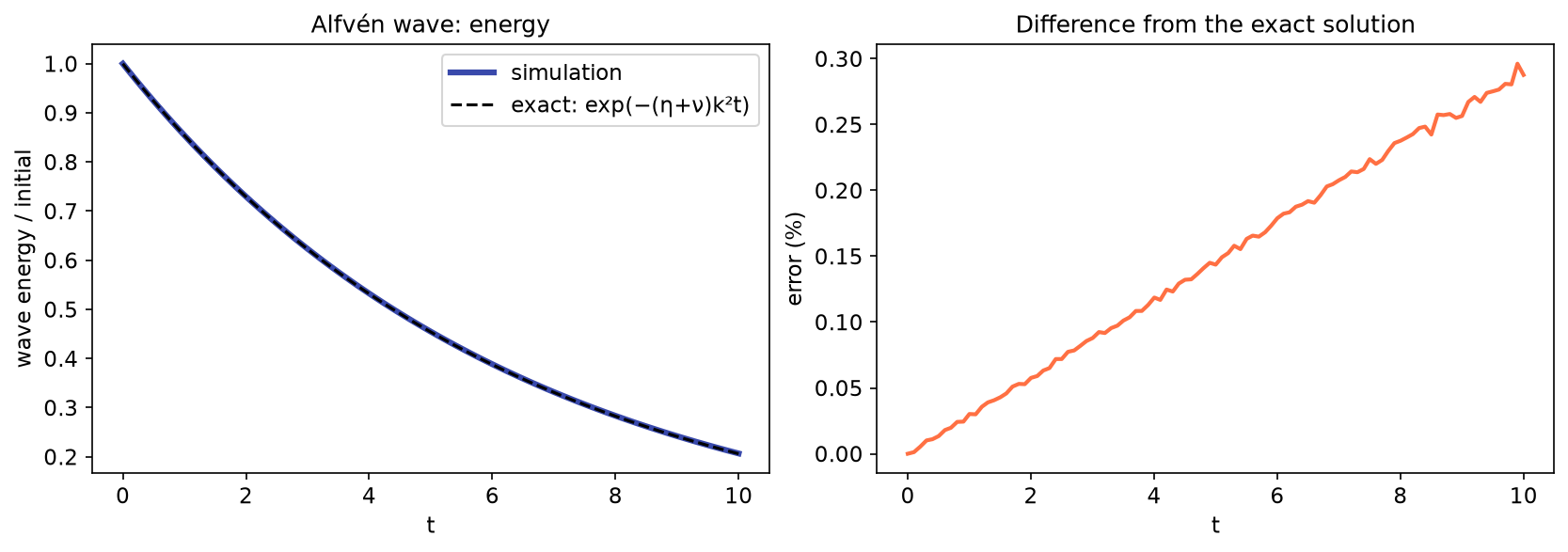
An exact solution. A small-amplitude Alfvén wave along a uniform field must keep its shape and lose energy as \(e^{-(\eta+\nu)k^2t}\) (derivation). The code agrees with this to 0.3%:

Conservation. With periodic or wall boundaries, mass and total energy (kinetic + magnetic + thermal + gravitational) should stay constant. The example runs keep mass to \(10^{-11}\) and energy to about 0.5% (the filter's dissipation is not returned as heat).

Constraints. \(\nabla\cdot\mathbf{B}\) stays at \(10^{-16}\) (round-off), as section 3 predicts.

The diagnostics are written to timeseries.csv and plotted by tools/plot_timeseries.py (Visualizing the results).

All the equations on one sheet

This is everything the code computes, in one place. Equations (1)–(4) are written out component by component for one cell \((i,j,k)\), with the physical terms, the numerical terms and the time step. Every abbreviation is defined in the table under the equations. Every quantity without indices is taken in the same cell \((i,j,k)\). The tabs show the same system in any coordinates (what the code does), in 2D Cartesian and in 2D spherical. Section 4 explains the equations one by one, and chart 4 shows the order in which they are computed.

Any coordinates, 3D (what the code computes)2D Cartesian \((x, y)\)2D spherical \((r, \theta)\)

The right-hand sides \(L(u)\): eight equations, one for each number stored in the cell.

\[ \begin{aligned} \frac{d\rho}{dt} &= -\frac{D_1(h_2h_3\,\rho v_1) + D_2(h_3h_1\,\rho v_2) + D_3(h_1h_2\,\rho v_3)}{h_1h_2h_3} - \mathcal F[\rho - \rho_0] + \epsilon\,\Delta_h(\rho - \rho_0) && (1) \\[10pt] \frac{dv_1}{dt} &= -\frac{D_1K}{h_1} + v_2\omega_3 - v_3\omega_2 - \frac{D_1p}{h_1\,\rho} + \frac{J_2B_3 - J_3B_2}{\rho} + g_1 + \nu\left[\frac43\,\frac{D_1\Theta}{h_1} - \frac{D_2(h_3\omega_3) - D_3(h_2\omega_2)}{h_2h_3}\right] - \mathcal F[v_1] && (2) \\[10pt] \frac{dv_2}{dt} &= -\frac{D_2K}{h_2} + v_3\omega_1 - v_1\omega_3 - \frac{D_2p}{h_2\,\rho} + \frac{J_3B_1 - J_1B_3}{\rho} + g_2 + \nu\left[\frac43\,\frac{D_2\Theta}{h_2} - \frac{D_3(h_1\omega_1) - D_1(h_3\omega_3)}{h_3h_1}\right] - \mathcal F[v_2] && (2) \\[10pt] \frac{dv_3}{dt} &= -\frac{D_3K}{h_3} + v_1\omega_2 - v_2\omega_1 - \frac{D_3p}{h_3\,\rho} + \frac{J_1B_2 - J_2B_1}{\rho} + g_3 + \nu\left[\frac43\,\frac{D_3\Theta}{h_3} - \frac{D_1(h_2\omega_2) - D_2(h_1\omega_1)}{h_1h_2}\right] - \mathcal F[v_3] && (2) \\[10pt] \frac{dp}{dt} &= -\frac{v_1D_1p}{h_1} - \frac{v_2D_2p}{h_2} - \frac{v_3D_3p}{h_3} - \gamma p\,\Theta + (\gamma-1)\Big[\eta\,|\mathbf J - \mathbf J_0|^2 + \rho\nu\big(|\boldsymbol\omega|^2 + \tfrac43\Theta^2\big) + \kappa\,\Delta_hT\Big] - \mathcal F[p - p_0] + \epsilon\,\Delta_h(p - p_0) && (3) \\[10pt] \frac{dA_1}{dt} &= v_2B_3 - v_3B_2 - \eta\,(J_1 - J_{0,1}) && (4) \\[4pt] \frac{dA_2}{dt} &= v_3B_1 - v_1B_3 - \eta\,(J_2 - J_{0,2}) && (4) \\[4pt] \frac{dA_3}{dt} &= v_1B_2 - v_2B_1 - \eta\,(J_3 - J_{0,3}) && (4) \end{aligned} \]

The abbreviations, each a formula for cell \((i,j,k)\):

Symbol	Definition	What it is
\(D_1, D_2, D_3\)	\((D_1f)_{i,j,k} = \dfrac{f_{i+1,j,k} - f_{i-1,j,k}}{2\Delta x_1}\), \((D_2f)_{i,j,k} = \dfrac{f_{i,j+1,k} - f_{i,j-1,k}}{2\Delta x_2}\), \((D_3f)_{i,j,k} = \dfrac{f_{i,j,k+1} - f_{i,j,k-1}}{2\Delta x_3}\)	central differences (§3); zero along a direction with one cell
\(h_1, h_2, h_3\)	Cartesian \((1, 1, 1)\); spherical \((1,\ r_i,\ r_i\sin\theta_j)\)	scale factors (§3)
\(B_1, B_2, B_3\)	\(B_1 = \dfrac{D_2(h_3A_3) - D_3(h_2A_2)}{h_2h_3} + B_{bg,1}\), \(B_2 = \dfrac{D_3(h_1A_1) - D_1(h_3A_3)}{h_3h_1} + B_{bg,2}\), \(B_3 = \dfrac{D_1(h_2A_2) - D_2(h_1A_1)}{h_1h_2} + B_{bg,3}\)	magnetic field \(\nabla_h\times\mathbf A + \mathbf B_{bg}\)
\(J_1, J_2, J_3\)	\(J_1 = \dfrac{D_2(h_3B_3) - D_3(h_2B_2)}{h_2h_3}\), \(J_2 = \dfrac{D_3(h_1B_1) - D_1(h_3B_3)}{h_3h_1}\), \(J_3 = \dfrac{D_1(h_2B_2) - D_2(h_1B_1)}{h_1h_2}\)	current \(\nabla_h\times\mathbf B\) (two cells each way from \(\mathbf A\))
\(\omega_1, \omega_2, \omega_3\)	\(\omega_1 = \dfrac{D_2(h_3v_3) - D_3(h_2v_2)}{h_2h_3}\), \(\omega_2 = \dfrac{D_3(h_1v_1) - D_1(h_3v_3)}{h_3h_1}\), \(\omega_3 = \dfrac{D_1(h_2v_2) - D_2(h_1v_1)}{h_1h_2}\)	vorticity \(\nabla_h\times\mathbf v\)
\(\Theta\)	\(\dfrac{D_1(h_2h_3v_1) + D_2(h_3h_1v_2) + D_3(h_1h_2v_3)}{h_1h_2h_3}\)	divergence \(\nabla_h\cdot\mathbf v\) (compression)
\(K\), \(T\)	\(K = \tfrac12(v_1^2 + v_2^2 + v_3^2)\), \(T = p/\rho\)	kinetic energy per mass, temperature
\(\lvert\boldsymbol\omega\rvert^2\), \(\lvert\mathbf J - \mathbf J_0\rvert^2\)	\(\omega_1^2 + \omega_2^2 + \omega_3^2\), \(\sum_{m}(J_m - J_{0,m})^2\)	for viscous and ohmic heating
\(\Delta_h f\)	\(\dfrac{1}{h_1h_2h_3}\left[D_1\!\Big(\dfrac{h_2h_3}{h_1}D_1f\Big) + D_2\!\Big(\dfrac{h_3h_1}{h_2}D_2f\Big) + D_3\!\Big(\dfrac{h_1h_2}{h_3}D_3f\Big)\right]\)	Laplacian \(\nabla_h\cdot\nabla_h f\) (two cells each way)
\(\mathcal F[f]\)	\(\dfrac{\sigma}{\Delta t^n}\big(\delta^4_1f + \delta^4_2f + \delta^4_3f\big)\), \((\delta^4_1f)_{i,j,k} = f_{i+2,j,k} - 4f_{i+1,j,k} + 6f_{i,j,k} - 4f_{i-1,j,k} + f_{i-2,j,k}\), likewise \(j\), \(k\)	filter of grid noise (§7); no \(\Delta x\): it works in cell units
\(\gamma, \eta, \nu, \kappa\)	config gamma (5/3), eta (a number, or \(\eta_{i,j,k}\) for localized resistivity), nu, kappa	physical constants (code units)
\(\epsilon, \sigma\)	config diffusion (default 0), filter (default 0.01)	numerical constants
\(\rho_0, p_0, \mathbf J_0, \mathbf B_{bg}, \mathbf g\)	initial \(\rho\) and \(p\); current of the initial equilibrium (0 unless sustain_equilibrium); uniform background field (Cartesian); gravity or applied force from the setup	fixed arrays, set once

The time step that uses them (sections 5 and 6):

\[ \begin{aligned} c_f &= \sqrt{\frac{\gamma p + B_1^2 + B_2^2 + B_3^2}{\rho}}, \qquad \chi = \max\!\Big(\max_{i,j,k}\eta,\ \nu,\ \epsilon,\ \frac{(\gamma-1)\,\kappa}{\min\rho}\Big) \\[8pt] \Delta t^n &= C\,\min\!\left[\ \min_{i,j,k,\ m}\ \frac{h_m\,\Delta x_m}{\sqrt{v_1^2 + v_2^2 + v_3^2} + c_f},\ \ \frac{\Delta x_{\min}^2}{2\,d\,\chi}\ \right] \quad\text{(and at most } t_{\text{end}} - t^n\text{)} \\[8pt] u^{(1)} &= u^n + \Delta t^n\,L(u^n) \\[4pt] u^{(2)} &= \tfrac34\,u^n + \tfrac14\Big[u^{(1)} + \Delta t^n\,L\big(u^{(1)}\big)\Big] \\[4pt] u^{n+1} &= \tfrac13\,u^n + \tfrac23\Big[u^{(2)} + \Delta t^n\,L\big(u^{(2)}\big)\Big] \end{aligned} \]

Here \(u = (\rho, v_1, v_2, v_3, p, A_1, A_2, A_3)\), \(L\) is the eight right-hand sides above in every physical cell, \(d\) is the number of dimensions and \(C\) the config cfl (0.4). After each of the three stages: \(\rho \leftarrow \max(\rho, \rho_{\text{floor}})\), \(p \leftarrow \max(p, p_{\text{floor}})\), and the ghost cells are filled (chart 5).

\(h = (1, 1, 1)\), cells \((i, j)\), and nothing varies along \(z\) (\(D_z = 0\)). The index \(k\) is dropped.

\[ \begin{aligned} \frac{d\rho}{dt} &= -D_x(\rho v_x) - D_y(\rho v_y) - \mathcal F[\rho - \rho_0] + \epsilon\,\Delta_h(\rho - \rho_0) && (1) \\[8pt] \frac{dv_x}{dt} &= -D_xK + v_y\omega_z - v_z\omega_y - \frac{D_xp}{\rho} + \frac{J_yB_z - J_zB_y}{\rho} + g_x + \nu\Big[\tfrac43 D_x\Theta - D_y\omega_z\Big] - \mathcal F[v_x] && (2) \\[8pt] \frac{dv_y}{dt} &= -D_yK + v_z\omega_x - v_x\omega_z - \frac{D_yp}{\rho} + \frac{J_zB_x - J_xB_z}{\rho} + g_y + \nu\Big[\tfrac43 D_y\Theta + D_x\omega_z\Big] - \mathcal F[v_y] && (2) \\[8pt] \frac{dv_z}{dt} &= v_x\omega_y - v_y\omega_x + \frac{J_xB_y - J_yB_x}{\rho} + g_z - \nu\big[D_x\omega_y - D_y\omega_x\big] - \mathcal F[v_z] && (2) \\[8pt] \frac{dp}{dt} &= -v_xD_xp - v_yD_yp - \gamma p\,\Theta + (\gamma-1)\Big[\eta\,|\mathbf J - \mathbf J_0|^2 + \rho\nu\big(|\boldsymbol\omega|^2 + \tfrac43\Theta^2\big) + \kappa\,\Delta_hT\Big] - \mathcal F[p - p_0] + \epsilon\,\Delta_h(p - p_0) && (3) \\[8pt] \frac{dA_x}{dt} &= v_yB_z - v_zB_y - \eta\,(J_x - J_{0,x}), \qquad \frac{dA_y}{dt} = v_zB_x - v_xB_z - \eta\,(J_y - J_{0,y}) && (4) \\[4pt] \frac{dA_z}{dt} &= v_xB_y - v_yB_x - \eta\,(J_z - J_{0,z}) && (4) \end{aligned} \]

Symbol	Definition in cell \((i,j)\)
\(D_x, D_y\)	\((D_xf)_{i,j} = \dfrac{f_{i+1,j} - f_{i-1,j}}{2\Delta x}\), \((D_yf)_{i,j} = \dfrac{f_{i,j+1} - f_{i,j-1}}{2\Delta y}\), \(D_z = 0\)
\(\mathbf B\)	\(B_x = D_yA_z + B_{bg,x}\), \(B_y = -D_xA_z + B_{bg,y}\), \(B_z = D_xA_y - D_yA_x + B_{bg,z}\)
\(\mathbf J\)	\(J_x = D_yB_z\), \(J_y = -D_xB_z\), \(J_z = D_xB_y - D_yB_x\)
\(\boldsymbol\omega\)	\(\omega_x = D_yv_z\), \(\omega_y = -D_xv_z\), \(\omega_z = D_xv_y - D_yv_x\)
\(\Theta\), \(K\), \(T\)	\(\Theta = D_xv_x + D_yv_y\), \(K = \tfrac12(v_x^2 + v_y^2 + v_z^2)\), \(T = p/\rho\)
\(\Delta_h f\)	\(D_xD_xf + D_yD_yf = \dfrac{f_{i+2,j} - 2f_{i,j} + f_{i-2,j}}{4\Delta x^2} + \dfrac{f_{i,j+2} - 2f_{i,j} + f_{i,j-2}}{4\Delta y^2}\)
\(\mathcal F[f]\)	\(\dfrac{\sigma}{\Delta t^n}\Big[\big(f_{i+2,j} - 4f_{i+1,j} + 6f_{i,j} - 4f_{i-1,j} + f_{i-2,j}\big) + \big(f_{i,j+2} - 4f_{i,j+1} + 6f_{i,j} - 4f_{i,j-1} + f_{i,j-2}\big)\Big]\)

Two equations with every difference written out. Continuity, and the induction equation for \(A_z\) (the one that carries the reconnection), with \(\mathbf B\) and \(\mathbf J\) put in from the table (\(J_z = -D_xD_xA_z - D_yD_yA_z\)):

\[ \begin{aligned} \frac{d\rho_{i,j}}{dt} &= -\frac{(\rho v_x)_{i+1,j} - (\rho v_x)_{i-1,j}}{2\Delta x} - \frac{(\rho v_y)_{i,j+1} - (\rho v_y)_{i,j-1}}{2\Delta y} \;-\; \mathcal F[\rho - \rho_0]_{i,j} \;+\; \epsilon\,\Delta_h(\rho - \rho_0)_{i,j} \\[10pt] \frac{d(A_z)_{i,j}}{dt} &= -(v_x)_{i,j}\left[\frac{(A_z)_{i+1,j} - (A_z)_{i-1,j}}{2\Delta x} - B_{bg,y}\right] - (v_y)_{i,j}\left[\frac{(A_z)_{i,j+1} - (A_z)_{i,j-1}}{2\Delta y} + B_{bg,x}\right] \\[6pt] &\quad + \eta\left[\frac{(A_z)_{i+2,j} - 2(A_z)_{i,j} + (A_z)_{i-2,j}}{4\Delta x^2} + \frac{(A_z)_{i,j+2} - 2(A_z)_{i,j} + (A_z)_{i,j-2}}{4\Delta y^2}\right] + \eta\,(J_{0,z})_{i,j} \end{aligned} \]

The first two terms of \(dA_z/dt\) carry the flux with the flow (\(\mathbf v\times\mathbf B\)); the bracket with \(\eta\) diffuses it, and is the only term that lets field lines reconnect.

\(h = (1, r, r\sin\theta)\), cells \((i, j)\) at \((r_i, \theta_j)\), nothing varies along \(\phi\) (\(D_\phi = 0\)). Because \(D_r\) compares cells at the same \(\theta_j\), a factor \(\sin\theta\) can be taken out of it, and \(r\) out of \(D_\theta\); this is how the general formulas shorten to the ones below.

\[ \begin{aligned} \frac{d\rho}{dt} &= -\frac{D_r(r^2\rho v_r)}{r^2} - \frac{D_\theta(\sin\theta\,\rho v_\theta)}{r\sin\theta} - \mathcal F[\rho - \rho_0] + \epsilon\,\Delta_h(\rho - \rho_0) && (1) \\[8pt] \frac{dv_r}{dt} &= -D_rK + v_\theta\omega_\phi - v_\phi\omega_\theta - \frac{D_rp}{\rho} + \frac{J_\theta B_\phi - J_\phi B_\theta}{\rho} + g_r + \nu\left[\tfrac43 D_r\Theta - \frac{D_\theta(\sin\theta\,\omega_\phi)}{r\sin\theta}\right] - \mathcal F[v_r] && (2) \\[8pt] \frac{dv_\theta}{dt} &= -\frac{D_\theta K}{r} + v_\phi\omega_r - v_r\omega_\phi - \frac{D_\theta p}{r\,\rho} + \frac{J_\phi B_r - J_rB_\phi}{\rho} + g_\theta + \nu\left[\frac43\,\frac{D_\theta\Theta}{r} + \frac{D_r(r\,\omega_\phi)}{r}\right] - \mathcal F[v_\theta] && (2) \\[8pt] \frac{dv_\phi}{dt} &= v_r\omega_\theta - v_\theta\omega_r + \frac{J_rB_\theta - J_\theta B_r}{\rho} + g_\phi - \nu\,\frac{D_r(r\,\omega_\theta) - D_\theta\omega_r}{r} - \mathcal F[v_\phi] && (2) \\[8pt] \frac{dp}{dt} &= -v_rD_rp - \frac{v_\theta D_\theta p}{r} - \gamma p\,\Theta + (\gamma-1)\Big[\eta\,|\mathbf J - \mathbf J_0|^2 + \rho\nu\big(|\boldsymbol\omega|^2 + \tfrac43\Theta^2\big) + \kappa\,\Delta_hT\Big] - \mathcal F[p - p_0] + \epsilon\,\Delta_h(p - p_0) && (3) \\[8pt] \frac{dA_r}{dt} &= v_\theta B_\phi - v_\phi B_\theta - \eta\,(J_r - J_{0,r}), \qquad \frac{dA_\theta}{dt} = v_\phi B_r - v_rB_\phi - \eta\,(J_\theta - J_{0,\theta}) && (4) \\[4pt] \frac{dA_\phi}{dt} &= v_rB_\theta - v_\theta B_r - \eta\,(J_\phi - J_{0,\phi}) && (4) \end{aligned} \]

Symbol	Definition in cell \((i,j)\), with \(r = r_i\), \(\theta = \theta_j\)
\(D_r, D_\theta\)	\((D_rf)_{i,j} = \dfrac{f_{i+1,j} - f_{i-1,j}}{2\Delta r}\), \((D_\theta f)_{i,j} = \dfrac{f_{i,j+1} - f_{i,j-1}}{2\Delta\theta}\), \(D_\phi = 0\)
\(\mathbf B\)	\(B_r = \dfrac{D_\theta(\sin\theta\,A_\phi)}{r\sin\theta}\), \(B_\theta = -\dfrac{D_r(r\,A_\phi)}{r}\), \(B_\phi = \dfrac{D_r(r\,A_\theta) - D_\theta A_r}{r}\) (no background field)
\(\mathbf J\)	\(J_r = \dfrac{D_\theta(\sin\theta\,B_\phi)}{r\sin\theta}\), \(J_\theta = -\dfrac{D_r(r\,B_\phi)}{r}\), \(J_\phi = \dfrac{D_r(r\,B_\theta) - D_\theta B_r}{r}\)
\(\boldsymbol\omega\)	\(\omega_r = \dfrac{D_\theta(\sin\theta\,v_\phi)}{r\sin\theta}\), \(\omega_\theta = -\dfrac{D_r(r\,v_\phi)}{r}\), \(\omega_\phi = \dfrac{D_r(r\,v_\theta) - D_\theta v_r}{r}\)
\(\Theta\), \(K\), \(T\)	\(\Theta = \dfrac{D_r(r^2v_r)}{r^2} + \dfrac{D_\theta(\sin\theta\,v_\theta)}{r\sin\theta}\), \(K = \tfrac12(v_r^2 + v_\theta^2 + v_\phi^2)\), \(T = p/\rho\)
\(\Delta_h f\)	\(\dfrac{D_r(r^2D_rf)}{r^2} + \dfrac{D_\theta(\sin\theta\,D_\theta f)}{r^2\sin\theta}\)
\(\mathcal F[f]\)	as in 2D Cartesian, in \(i\) and \(j\) (cell units, so the same formula)
\(\mathbf g\)	from the setup: \(g_r = -GM/r^2\) for the corona, or the applied push of the dipole runs

Continuity with every difference written out (the products are formed in the neighbouring cells):

\[ \frac{d\rho_{i,j}}{dt} = -\frac{(r^2\rho v_r)_{i+1,j} - (r^2\rho v_r)_{i-1,j}}{2\Delta r\; r_i^2} - \frac{(\sin\theta\,\rho v_\theta)_{i,j+1} - (\sin\theta\,\rho v_\theta)_{i,j-1}}{2\Delta\theta\; r_i\sin\theta_j} - \mathcal F[\rho - \rho_0]_{i,j} + \epsilon\,\Delta_h(\rho - \rho_0)_{i,j} \]

The code has no separate spherical formulas: the general lines of section 3 produce these from the arrays \(h_m\).

The algorithm as flow charts

Chart 1 is the whole run. Charts 2–5 each open up one method that chart 1 calls: the time step, one RK3 step, one evaluation of the right-hand side (where the equation sheet is computed) and the ghost cells. Every box is a link to the place on this page where it is explained.

■ input  ■ set up / ghost cells  ■ time loop  ■ equations  ■ output  ■ stop

Chart 1: the whole run

run in solver.py. Before each step the loop checks what is due (diagnostics, snapshot, end), then takes one step.

The same as pseudo-code, and in the notation of this page

read config  →  build grid (cells, ghost cells, h1 h2 h3)
set initial state (rho, v, p, A)  →  fill ghost cells
repeat until t = t_end:
    dt = CFL * min(cell width / (|v| + fast speed),  cell width² / (2 d diffusivity))
    three Runge–Kutta stages, each:
        B = curl A,  J = curl B,  w = curl v
        evaluate the right-hand sides of rho, v, p, A (with the filter)
        update the physical cells  →  apply floors  →  fill ghost cells
    every dt_diag:   write energies, flux, max |J|, div B to timeseries.csv
    every dt_output: write a snapshot (rho, p, v, A, B, J, E) to snap_XXXX.npz

For one step \(n \to n+1\):

1. \(\Delta t^n = C\min\big[\min_{i,j,k,m} h_m\Delta x_m/(|\mathbf v| + c_f),\ \Delta x_{\min}^2/(2d\chi)\big]\) (CFL).
2. For each stage \(s = 1, 2, 3\), with input \(u^n\), \(u^{(1)}\), \(u^{(2)}\):
   1. \(\mathbf B = \nabla_h\times\mathbf A + \mathbf B_{bg}\), \(\mathbf J = \nabla_h\times\mathbf B\), \(\boldsymbol\omega = \nabla_h\times\mathbf v\) (the chain);
   2. \(L_\rho, L_{\mathbf v}, L_p, L_{\mathbf A}\) in every physical cell, the equation sheet;
   3. the Runge–Kutta combination for every physical cell (RK3);
   4. floors on \(\rho, p\), then fill the ghost cells.
3. \(t^{n+1} = t^n + \Delta t^n\); write diagnostics and snapshots when due.

Chart 2: the time step Δt (CFL condition)

timestep in solver.py: two limits, waves (left) and diffusion (right), and the stricter one wins. Explained in the CFL condition.

Chart 3: one RK3 step

rk3_step in solver.py: three evaluations of \(L\), each followed by the floors and the ghost cells. Explained in third-order Runge–Kutta.

Chart 4: the right-hand side L(u)

rhs in physics.py: the chain of section 4, from the stored \(u\) to the eight right-hand sides of the equation sheet. Each row is valid one cell less far into the ghost layers.

Chart 5: the ghost cells

fill_ghosts in boundaries.py, after the initial state and after every RK3 stage. Explained in section 5.

The same, animated

Cell by cell on a coarse 14 × 8 grid with the solver's own numbers (the steps in words):

Jump to:1. Grid2. Ghost cells3. Initial state4. Fill ghosts5. Time step6. Equations7. RK3 & loop8. Repeatspeed 0.5×0.75×1×1.5×

Practice problems

Try each problem before opening its solution. Click an option to check a concept question; type a number and press Check for a numerical one (forms like 6.2e7 or 6.2x10^7 both work).

Concept questions

Problem 1

Why does the code evolve the vector potential \(\mathbf{A}\) instead of \(\mathbf{B}\)?

• It needs fewer grid points
• \(\mathbf{B} = \nabla\times\mathbf{A}\) keeps \(\nabla\cdot\mathbf{B} = 0\) automatically, even on the grid
• \(\mathbf{A}\) is gauge invariant
• Resistivity cannot be included in an equation for \(\mathbf{B}\)

The discrete divergence of a discrete curl vanishes because central differences in different directions commute, so no magnetic monopoles are created.

Problem 2

A 3D grid has 1 cell in the \(z\) direction. What does the code do?

• It stops with an error
• It treats \(z\) as periodic with one cell
• It treats \(z\) as invariant: \(\partial_z = 0\), but vectors keep their \(z\) components
• It ignores the \(z\) components of all vectors

A direction with one cell is invariant. This is how the same code runs 2D (strictly, 2.5D) problems with an out-of-plane current or guide field.

Problem 3

What limits the time step of a spherical run with \(r\in[1, 5]\)?

• The smallest physical cell, \(r\Delta\theta\) or \(r\sin\theta\Delta\phi\) at the inner radius
• The largest cell, at the outer radius
• The number of snapshots
• The radial cell size \(\Delta r\) alone

The CFL condition must hold in every cell. The angular cells are smallest at small \(r\), where the field (and the fast speed) is also strongest.

Problem 4

Why is the filter not applied to \(\mathbf{A}\)?

• \(\mathbf{A}\) never has grid noise
• Filtering \(\mathbf{A}\) would act like an extra (hyper)resistivity and change the reconnection rate
• It would break \(\nabla\cdot\mathbf{B} = 0\)
• \(\mathbf{A}\) has no ghost cells

Any diffusion of \(\mathbf{A}\) lets field lines slip through the plasma, which is reconnection. Keeping \(\mathbf{A}\) unfiltered means the only cause of reconnection is the physical \(\eta\) you chose.

Show that…

Problem 5: second-order accuracy

Show that \((f_{i+1} - f_{i-1})/(2\Delta x)\) differs from \(f'(x_i)\) by \(\tfrac16\Delta x^2 f'''(x_i)\) plus higher-order terms.

Hint

Write the Taylor series of \(f_{i+1}\) and \(f_{i-1}\) up to the third derivative and subtract.

Proof

\(f_{i+1} - f_{i-1} = 2\Delta x f' + \tfrac13\Delta x^3 f''' + O(\Delta x^5)\), because the even terms cancel. Dividing by \(2\Delta x\): \(f' + \tfrac16\Delta x^2 f''' + O(\Delta x^4)\).

Problem 6: forward Euler is unstable

For \(du/dt = i\omega u\) (a pure oscillation, \(\omega\) real), show that forward Euler multiplies \(|u|\) by \(\sqrt{1 + \omega^2\Delta t^2} > 1\) every step.

Hint

\(u^{n+1} = (1 + i\omega\Delta t)u^n\). Take the modulus.

Proof

\(|1 + i\omega\Delta t| = \sqrt{1 + \omega^2\Delta t^2}\), which exceeds 1 for any \(\Delta t > 0\). After \(N\) steps the error has grown by \((1+\omega^2\Delta t^2)^{N/2}\), however small \(\Delta t\) is.

Problem 7: what the filter does to a wave

Show that for a wave \(f_i = e^{\mathrm{i}kx_i}\) (\(k\) the wavenumber, \(\mathrm{i} = \sqrt{-1}\), \(x_i\) the cell centres), \(f_{i+2} - 4f_{i+1} + 6f_i - 4f_{i-1} + f_{i-2} = 16\sin^4(k\Delta x/2)\,f_i\).

Hint

The operator is the square of the second difference \(f_{i+1} - 2f_i + f_{i-1}\). What does that give for \(e^{ikx}\)?

Proof

\(f_{i+1} - 2f_i + f_{i-1} = (e^{ik\Delta x} - 2 + e^{-ik\Delta x})f_i = -4\sin^2(k\Delta x/2)\,f_i\). Applying it twice gives \(16\sin^4(k\Delta x/2)\,f_i\), and expanding \((f_{i+1} - 2f_i + f_{i-1})\) twice gives the five-point formula.

Numbers

Problem 8

A Cartesian 2D run has \(\Delta x = 0.1\) and a fastest signal \(|v| + c_f = 2.5\). With CFL number 0.4, what is the time step?

Solution

\(\Delta t = 0.4\times0.1/2.5 = 0.016\), close to the \(1.6\times10^{-2}\) the Harris run reports.

Problem 9

How many time steps does that run need to reach \(t = 200\)?

Solution

\(200/0.016 = 12\,500\). Each step costs three evaluations of the right-hand side.

Problem 10

The same grid has \(\eta = \nu = 0.005\). What is the diffusive time-step limit \(\Delta x^2/(2d\,\eta)\) in 2D (before the CFL factor)?

Solution

\(0.01/(2\times2\times0.005) = 0.01/0.02 = 0.5\). This is 12 times larger than the wave limit (\(0.1/2.5 = 0.04\)), so waves, not diffusion, set the time step.

Problem 11

You double the resolution of a 3D run in every direction. By what factor does the run time grow?

Solution

\(2^3 = 8\) times more cells, and the time step halves (CFL), so twice as many steps: \(8\times2 = 16\). In 2D the factor is \(4\times2 = 8\).