Spherical runs (2D and 3D)¶

Planets and stars are round. Near them, magnetic fields fall off with distance (a dipole as \(1/r^3\)), and spherical coordinates \((r, \theta, \phi)\) follow that geometry: the planet's surface is simply \(r = r_{\text{in}}\). The same solver handles them. Only the scale factors change, \((h_r, h_\theta, h_\phi) = (1, r, r\sin\theta)\) (why that is enough).

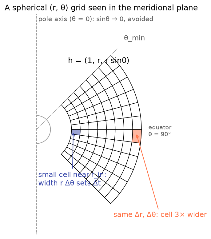
A spherical grid in the meridional plane

Three things are different from a Cartesian box:

Cells grow with radius. With fixed \(\Delta r\) and \(\Delta\theta\), a cell at \(r = 3\) is three times wider than one at \(r = 1\). The resolution is best near the inner boundary, and so is the field strength, so the time step is set there.
The poles are avoided. At \(\theta = 0\) and \(\pi\), \(\sin\theta = 0\) and the operators divide by zero. The domain stops at \(\theta_{\min} > 0\) with walls. Codes that include the poles need special treatment there.
2D means axisymmetric. A grid with one cell in \(\phi\) describes a system that looks the same at every longitude: each point of the 2D picture is really a ring around the axis.

Build your run¶

Choose the setup and the dimensions, change any parameter, and press Download config file. The file goes to your Downloads folder; start the lab and it is listed under Your configs (how to start the lab).

See it before you run it. Above the form is a picture of the chosen setup at \(t = 0\): the magnetic field (in 3D with arrows and field lines), the current, the plasma and the push that starts the run, with what will happen. It is drawn with the example's parameters. Preview script downloads a small Python file that draws the same picture with your parameters: run python3 ~/Downloads/preview_<name>.py (add --html for a 3D page you can rotate). Or type show in the lab before you press Return.

How the code runs¶

The chart follows one run from the config file to the pictures. The boxes in the dashed frames repeat every time step. Click any box to read how that step is done. The live monitor lights up the same stages while your run is going.

Setup 1: a magnetosphere with a magnetic null¶

The field¶

Put a dipole (a planet) inside a uniform field pointing the opposite way at the equator. This is Earth's magnetosphere when the interplanetary field turns southward, the situation in which Dungey (1961) proposed that reconnection drives the whole magnetosphere. In code units the flux function is

\[ \Psi = r\sin\theta\,A_\phi = \sin^2\theta\left(\frac{1}{r} + \frac{b\,r^2}{2}\right), \]

whose two terms are the dipole (strength 1) and a uniform field of strength \(b\). Using \(B_r = \partial_\theta\Psi/(r^2\sin\theta)\) and \(B_\theta = -\partial_r\Psi/(r\sin\theta)\):

\[ B_r = \cos\theta\left(\frac{2}{r^3} + b\right), \qquad B_\theta = \sin\theta\left(\frac{1}{r^3} - b\right). \]

On the equator \(B_r = 0\), and \(B_\theta\) changes sign at

\[ \boxed{\;r_{\text{null}} = b^{-1/3}\;} \]

where the dipole's field and the uniform field cancel. That circle is a magnetic null: an X-line bent into a ring around the planet. Its separatrix (orange below) divides space into three kinds of field line: closed lines with both ends on the planet, open lines with one end on the planet, and external lines that never touch it.

Equilibrium for free. The field is a sum of a dipole and a uniform field, both curl-free, so \(\mathbf{J} = 0\) and there is no magnetic force at all. Uniform density and pressure are then an exact equilibrium. No gravity is needed.

Driving¶

A current-free field has no free energy to release. Something has to push. The code adds a steady force per unit mass on the equator outside the null, pointing inward,

\[ a_r = -a_0\,e^{-(\Theta/w_\theta)^2}\,e^{-((r - r_d)/w)^2}, \qquad \Theta = \tfrac{\pi}{2} - \theta, \]

a stand-in for solar-wind pressure on the dayside. In 3D it is multiplied by \((1 - \cos m\phi')/2\), so the push acts on \(m\) patches of longitude. Alternatively, an initial inflow pulse v0 can kick the null once.

splmhd/setups.py

def dipole_null(grid, prm):
    """A dipole inside a uniform, antiparallel field: a magnetosphere in a box.

    Flux function Psi = r sin(theta) A_phi = sin^2(theta) (1/r + b r^2/2), with b = 1/r_null^3:
        B_r     = 2 cos(theta)/r^3 + b cos(theta)
        B_theta = sin(theta) (1/r^3 - b)
    The dipole's equatorial field and the uniform field cancel on the ring r = r_null:
    a magnetic null (an X-line bent into a circle), like the dayside magnetopause
    when the interplanetary field is antiparallel to Earth's field (Dungey 1961).
    The field is current-free, so uniform rho and p make an exact equilibrium.
    Reconnection is driven in one of two ways (either can be zero):
      an initial inflow pulse towards the null from both sides,
        v_r = -v0 tanh((r - r_null)/w) exp(-(Theta/w_theta)^2)       [x (1 - cos m phi')/2 in 3D]
      and a steady push from outside, like solar-wind pressure on the dayside magnetopause,
        a_r = -drive exp(-(Theta/w_theta)^2) exp(-((r - r_d)/w)^2),  r_d = (r_null + r_out)/2
    """
    if grid.geometry != "spherical":
        raise ValueError("the dipole setup needs spherical geometry")
    r_null = prm.get("r_null", 2.0)
    v0 = prm.get("v0", 0.3)
    w = prm.get("width_r", 0.5)
    w_th = prm.get("width_theta", 0.3)
    m_phi = prm.get("m_phi", 1)
    b = 1.0 / r_null**3
    r, th, ph = grid.X
    Th = np.pi / 2 - th

    s = _blank(grid)
    s["rho"][:] = prm.get("rho", 1.0)
    s["p"][:] = prm.get("p", 0.05)
    s["A"][2] = np.sin(th) * (1.0 / r**2 + 0.5 * b * r)
    A_eq = s["A"].copy()
    pulse = np.exp(-(Th / w_th) ** 2)
    if grid.active[2]:
        Lphi = grid.hi[2] - grid.lo[2]
        pulse = pulse * 0.5 * (1 - np.cos(2 * np.pi * m_phi * (ph - grid.lo[2]) / Lphi))  # patch mid-wedge
    s["v"][0] = -v0 * np.tanh((r - r_null) / w) * pulse * np.exp(-((r - r_null) / (3 * w)) ** 2)
    extra = {"B_bg": np.zeros(3), "A_eq": A_eq, "flux_kind": "xpoint", "eta_center": r_null}
    drive = prm.get("drive", 0.0)
    if drive > 0:
        r_d = 0.5 * (r_null + grid.hi[0])
        force = np.zeros((3,) + grid.shape)
        force[0] = -drive * pulse * np.exp(-((r - r_d) / w) ** 2)
        extra["gravity"] = force  # a body force per unit mass, handled like gravity
        extra["potential"] = None
    return s, extra

Boundaries. fixed (line-tied) at both radial boundaries, conducting walls in \(\theta\), periodic in \(\phi\). A fixed boundary holds density and pressure at their initial values, so it acts as a reservoir: a few percent of the mass can flow in or out over a run, like plasma exchanged with a dense ionosphere or photosphere.

What happens¶

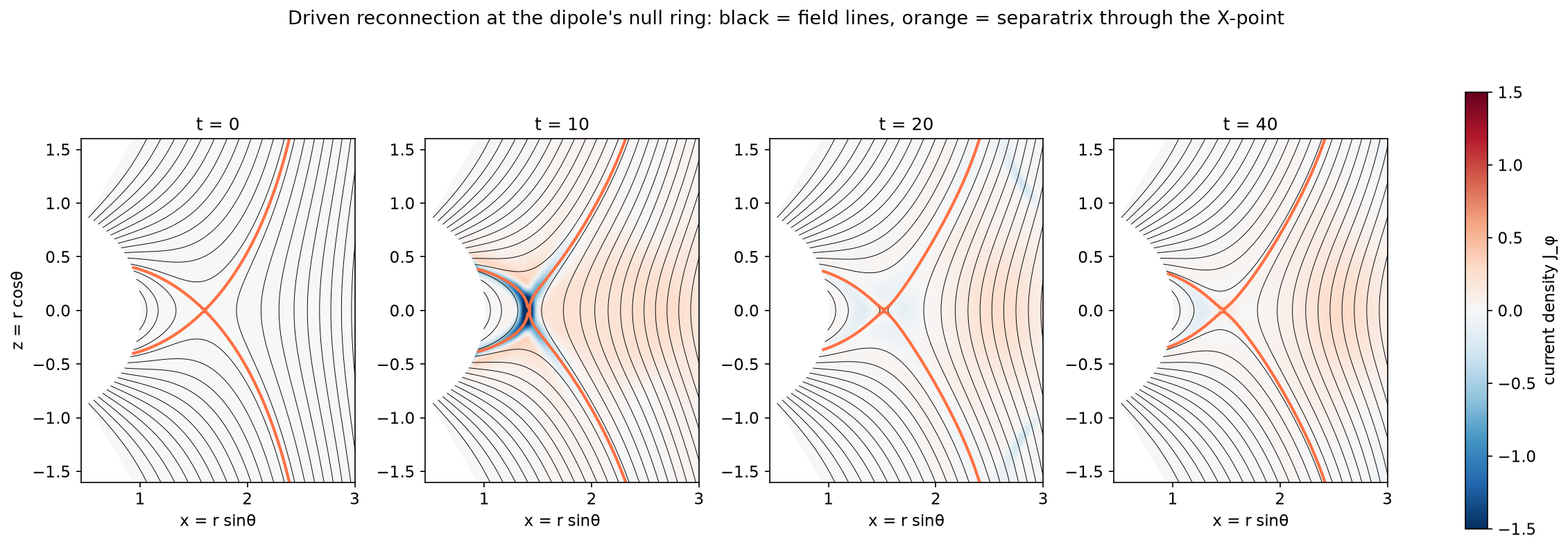
Driven reconnection at the null ring

spherical_2d_dipole (\(160\times128\) cells, \(\eta = \nu = 10^{-3}\), about 2 minutes):

\(t = 0\). The X-point sits on the equator at \(r = 1.6\).
Collapse (\(t\approx10\)). The push squeezes the X-point. The null cannot stay a simple cross: it collapses into a short, intense current sheet (dark blue) along the separatrix. This is X-point collapse, the 2D way a stressed null releases energy.
Reconnection. In the sheet, external field lines reconnect with closed dipole field lines, which is the magnetospheric version of the field-line journey on the advanced pages. The separatrix moves and the X-point settles closer to the planet (\(r\approx1.45\)), where the stronger dipole field can balance the push.

Reconnected flux at the null

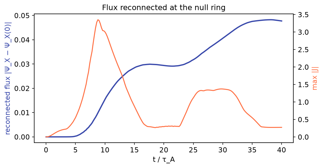
The reconnected flux grows in steps. The current sheet forms, reconnects flux and relaxes, the push stresses the null again, and so on. Real magnetospheres show the same bursty behaviour.

In 3D: reconnection on part of the ring¶

In spherical_3d_dipole (a \(180°\) wedge in \(\phi\), \(m = 1\)) the push acts only around the middle of the wedge, \(\phi\approx90°\). The left panel measures the flux reconnected at the null ring at each longitude (the change of \(\Psi\) at the X-point); the right panel shows the current \(J_\phi\) in the equatorial plane, seen from above the pole:

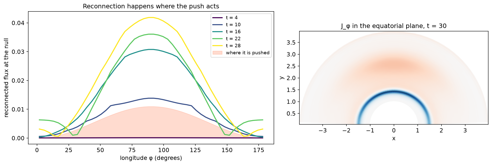
Reconnected flux against longitude in the 3D dipole run

Reconnection is concentrated where the field is pushed: by \(t = 30\) the flux reconnected at \(\phi = 90°\) is about ten times that at the edges of the wedge. This is a simple model of patchy dayside reconnection, like the flux-transfer events seen at Earth's magnetopause.

Experiments to try¶

1. Push harder or softer

Change the steady push between 0.02 and 0.1. Does the reconnected flux grow in proportion? Does the X-point move further in?

2. A one-off kick instead of a steady push

Set the push to 0 and the initial inflow pulse to 0.3. The null collapses, reconnects, then the flux flows back: oscillatory reconnection, a ringing of the null that is studied as a source of quasi-periodic pulsations in solar flares.

3. Move the null

Change the null radius between 1.3 and 2.5. The weaker the field at the null, the slower the Alfvén speed there, and the slower the reconnection.

4. Patches in 3D

In 3D, set patches around φ to 2 or 3 and compare with one patch. Do neighbouring patches merge?

Setup 2 (advanced): a current sheet in a gravitating corona¶

This setup is a lesson in why spherical geometry, gravity and equilibrium are harder than they look.

A split monopole, \(B_r = \tanh(\Theta/\Delta)/r^2\), points outward in the north and inward in the south, with a current sheet at the equator. It is the simplest model of the heliospheric current sheet or a coronal streamer. Two balances are needed:

Across the sheet, \(p + B_r^2/2\) must not depend on \(\theta\), as in the Harris sheet. Because \(B_r^2\propto r^{-4}\), the pressure in the sheet must fall as \(r^{-4}\).
Along \(r\), a pressure falling as \(r^{-4}\) pushes outward, so something must pull inward: gravity, \(dp/dr = -\rho\,GM/r^2\).

Both hold exactly for

\[ p = \frac{\beta + \operatorname{sech}^2(\Theta/\Delta)}{2r^4}, \qquad \rho = \frac{2\left[\beta + \operatorname{sech}^2(\Theta/\Delta)\right]}{GM\,r^3}, \qquad T = \frac{p}{\rho} = \frac{GM}{4r}. \]

splmhd/setups.py

def spherical_sheet(grid, prm):
    """A current sheet at the equator of a gravitating, stratified corona.

    B_r = tanh(Theta/delta) / r^2 with Theta = pi/2 - theta: a split monopole,
    like the heliospheric current sheet. Equilibrium needs
        across the sheet:  p + B_r^2/2 independent of theta
        along r:           dp/dr = -rho GM/r^2
    Both hold for
        p   = (beta + sech^2(Theta/delta)) / (2 r^4)
        rho = 2 (beta + sech^2(Theta/delta)) / (GM r^3),   T = p/rho = GM/(4r).
    The flux function Psi = r sin(theta) A_phi depends only on theta (radial field lines);
    the perturbation dPsi = psi0 sin(n pi (r - r_in)/(r_out - r_in)) exp(-(Theta/(3 delta))^2)
    cos(m phi') seeds tearing (m = 0: axisymmetric).
    """
    if grid.geometry != "spherical":
        raise ValueError("the spherical-sheet setup needs spherical geometry")
    delta = prm.get("delta", 0.05)
    beta = prm.get("beta", 0.5)
    GM = prm.get("GM", 4.0)
    psi0 = prm.get("psi0", 2e-3)
    n_r = prm.get("n_r", 4)
    m_phi = prm.get("m_phi", 1)
    r, th, ph = grid.X
    Th = np.pi / 2 - th
    sech2 = 1.0 / np.cosh(Th / delta) ** 2

    s = _blank(grid)
    s["p"] = (beta + sech2) / (2 * r**4)
    s["rho"] = 2 * (beta + sech2) / (GM * r**3)

    # Psi(theta) = integral of tanh((pi/2-theta')/delta) sin(theta') d theta' from pi/2
    tfine = np.linspace(grid.x[1][0], grid.x[1][-1], 20001)
    integrand = np.tanh((np.pi / 2 - tfine) / delta) * np.sin(tfine)
    F = np.concatenate([[0], np.cumsum(0.5 * (integrand[1:] + integrand[:-1]) * np.diff(tfine))])
    F -= np.interp(np.pi / 2, tfine, F)
    Psi = np.interp(th, tfine, F)

    r_in, r_out = grid.lo[0], grid.hi[0]
    pert = psi0 * np.sin(n_r * np.pi * (r - r_in) / (r_out - r_in)) * np.exp(-(Th / (3 * delta)) ** 2)
    if grid.active[2]:
        Lphi = grid.hi[2] - grid.lo[2]
        pert = pert * np.cos(2 * np.pi * m_phi * (ph - grid.lo[2]) / Lphi)
    s["A"][2] = (Psi + pert) / (r * np.sin(th))
    A_eq = np.zeros_like(s["A"])
    A_eq[2] = Psi / (r * np.sin(th))

    gravity = np.zeros((3,) + grid.shape)
    gravity[0] = -GM / r**2
    return s, {"B_bg": np.zeros(3), "gravity": gravity, "potential": -GM / r, "A_eq": A_eq}

What we found while building this setup (you can reproduce each step):

The sheet diffuses before it tears. Near \(r = 1\) the sheet is thin and the current strong. With \(\eta = 2\times10^{-4}\) it diffuses in about 50 time units, and ohmic heating makes the hot sheet plasma rise against gravity. Switching on sustain equilibrium adds the applied field \(\mathbf{E}_0 = \eta\mathbf{J}_0\) of tearing-mode studies, which holds the initial current in place so that only the perturbation evolves.
Short wavelengths do not tear. A tanh sheet of half-thickness \(a\) is unstable to tearing only for \(ka < 1\). Six half-waves along \(r\in[1,5]\) give \(ka\approx1.4\): stable. The default uses two.
Gravity resists tearing. The equilibrium forces a scale height \(H = T/g = r/4\): density drops 125-fold from \(r = 1\) to 5. Tearing needs flows along the sheet, here up and down in \(r\), against this strong stratification. In our tests the islands grew only slowly (e-folding times above 50), much more slowly than a Harris sheet with the same Lundquist number.

That is why this setup is the "advanced" one. Try lowering the gravity (GM) and see whether the sheet tears faster. Note that the temperature then falls too, since \(T = GM/4r\).

Practice problems¶

Try each problem before opening its solution. Click an option to check a concept question; type a number and press Check for a numerical one (forms like 6.2e7 or 6.2x10^7 both work).

Concept questions¶

Problem 1

Why does the spherical domain stop short of the poles?

The field is zero at the poles
\(\sin\theta = 0\) there, so the operators divide by zero and the cells shrink to nothing
Reconnection never happens at the poles
Periodic boundaries cannot be used in \(\theta\)

The scale factor \(h_\phi = r\sin\theta\) vanishes at the poles. Divisions by \(r\sin\theta\) blow up, and the time step (set by the smallest cell, \(r\sin\theta\Delta\phi\)) would go to zero in 3D.

Problem 2

Why is a dipole plus a uniform field an equilibrium with uniform pressure?

Both fields are curl-free, so \(\mathbf{J} = 0\) and there is no magnetic force
The two fields cancel everywhere
Gravity balances the magnetic force
The magnetic pressure is uniform

\(\mathbf{J} = \nabla\times\mathbf{B} = 0\) for both, so \(\mathbf{J}\times\mathbf{B} = 0\). With no force from the field, uniform \(p\) and \(\rho\) balance trivially. The field is not uniform, but a force-free field exerts no net force.

Problem 3

What does a 2D (axisymmetric) spherical run assume?

That the field has no \(\phi\) component
That the system is a thin slice of a sphere
That nothing depends on longitude \(\phi\): each point is a ring around the axis
That the problem is 2D Cartesian

\(\partial_\phi = 0\) everywhere, but vectors keep their \(\phi\) components (for example \(J_\phi\), the ring current of the null). The null itself is a ring.

Show that…¶

Problem 4: the null radius

From \(B_\theta = \sin\theta\,(1/r^3 - b)\) on the equator, show that the null lies at \(r = b^{-1/3}\), and that \(b = 1/8\) puts it at \(r = 2\).

Hint

On the equator \(B_r = 0\) already. Set \(B_\theta = 0\).

Proof

\(1/r^3 = b\Rightarrow r = b^{-1/3}\). For \(b = 1/8\), \(r = 8^{1/3} = 2\).

Problem 5: the corona's temperature

Show that \(p\) and \(\rho\) of Setup 2 satisfy \(dp/dr = -\rho GM/r^2\), and that \(T = p/\rho = GM/(4r)\).

Hint

Write \(p = Q/(2r^4)\) and \(\rho = 2Q/(GMr^3)\) with \(Q = \beta + \operatorname{sech}^2(\Theta/\Delta)\), which does not depend on \(r\).

Proof

\(dp/dr = -4Q/(2r^5) = -2Q/r^5\). And \(\rho GM/r^2 = (2Q/(GMr^3))(GM/r^2) = 2Q/r^5\). So \(dp/dr = -\rho GM/r^2\). Then \(T = p/\rho = [Q/(2r^4)]\,[GMr^3/(2Q)] = GM/(4r)\).

Numbers¶

Problem 6

With \(b = 0.244\) (null at \(r = 1.6\)), what is the dipole field strength \(|B_\theta| = 1/r^3\) on the equator at the null? (It is cancelled exactly by the uniform field.)

Solution

\(1/1.6^3 = 1/4.096 = 0.244 = b\), as it must be at the null.

Problem 7

A spherical grid has \(\Delta\theta = 1°\), and \(r\) runs from 1 to 4. How many times wider is a cell at the outer boundary than at the inner one, in the \(\theta\) direction?

Solution

The width is \(r\Delta\theta\), so the ratio is \(4/1 = 4\). Fine structure far from the planet is resolved four times worse than near it.

Problem 8

For the corona of Setup 2, what is the density scale height \(H = r/4\) at \(r = 2\), in units of the inner radius?

Solution

\(H = 2/4 = 0.5\). A tearing mode with wavelength 4 along \(r\) spans eight scale heights, so its flows run steeply uphill.